Sometimes, algorithms look biased but might not be, and other times algorithms look unbiased but may be - how can you tell?

The detection of bias in algorithms is an important capability to ensure your algorithms are treating your customers fairly, and to make sure your organisation is acting ethically and within the legal bounds of anti-discrimination legislation.

It is important to note up front that not all bias is bad - directing appropriate marketing to subgroups of people (e.g. nappies to the parents of newborns) can improve their customer experience and provide them with better services based on personalisation for their specific needs. However, there are many examples of bias which are unfair and in some cases potentially illegal, such as gender or ethnicity. It is important to have reliable methods of determining if a bias is present and understanding the confidence of that determination.

There also are many different types of bias and fairness. A good introduction to the definitions of different types of fairness is given by Ziyuan Zhong in his Tutorial on Fairness in Machine Learning.

This blog is concerned with the measurement of the bias in recommendations, classification and outcomes, rather than with the source of bias which may come from either the data or the algorithms themselves (see this blog post for more detail on this).

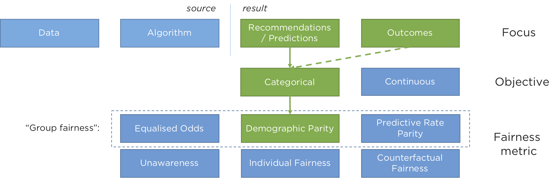
All of the examples we give below concern the measurement of “demographic parity” or “statistical parity” - the most commonly understood notion of group fairness, and for systems where algorithms choose between a finite number of outcomes (rather than optimising a continuous variable). This means we can make judgements using the techniques we explain here about the algorithms that decide whether or not someone is offered credit (a binary, categorical decision) rather than the amount of credit being offered (a continuous variable).

We (Ambiata) do this because we build systems that make recommendations for customers, and essentially we are concerned with understanding whether or not the rate we make recommendations to one sub-group is significantly different to the rest of the population. If it is, we have a bias, and in some cases, that bias would be considered unfair, or at worse, illegal.

In this post, we will give a simple example, illustrate some methods of bias measurement and alerting, evaluate them, and then drop into the maths that makes them work.

An example

Imagine you are running an automated decisioning system to make customer recommendations. You want to check if your decisioning system is making biased decisions between one group compared to the rest of the population. This is a harder problem than it should be because of random sampling effects.

Just say you had a population of that consists of an equal number of city folk and country folk. If you have an algorithm that offered a discount to people based on where they lived, amongst other characteristics, and the algorithms choose to send discounts to 25 out of 100 city folk and 20 out of 110 country folk.

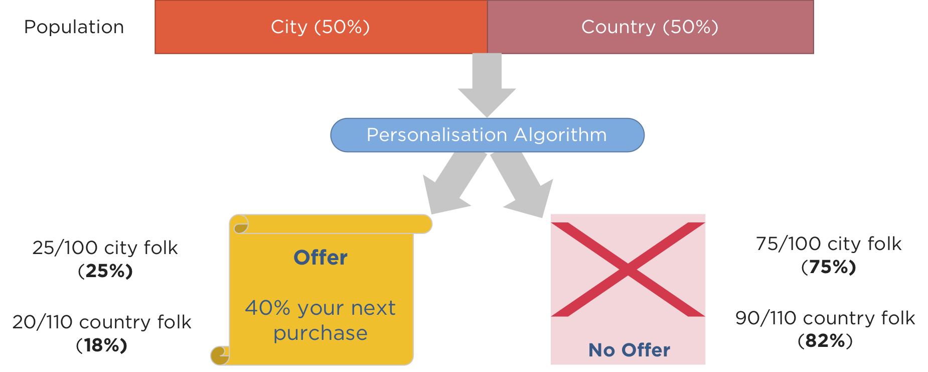
Is this an example of an intrinsically biased algorithm? On the surface it looks like it, as a smaller proportion of country folk (18%) get offered a discount compared to city folk (25%).

Unfortunately, this is a much more subtle problem than it first appears. In fact, this is similar to the question as to whether a coin is biased if you observe it flip heads 7 out of 10 times, say. Clearly you have some evidence to suggest it is biased, but are you sure? You know that some proportion of the times you flip an unbiased coin 10 times, it will come up heads 7 times at least a few of them. Random chance affects the significance of the result.

To illustrate this, consider a simulation where the algorithm is unbiased - it chooses to send 22% of folk a discount, regardless of whether they are in the city or the country. Let’s do this over and over - 100,000 times, sending offers randomly at a rate of 22%, to 100 city folk and 110 country folk, and draw the histogram of how often each set of numbers of offers is chosen. In this simulation, the algorithm will, on average, give 22 offers to the city folk and 24 offers to the country folk.

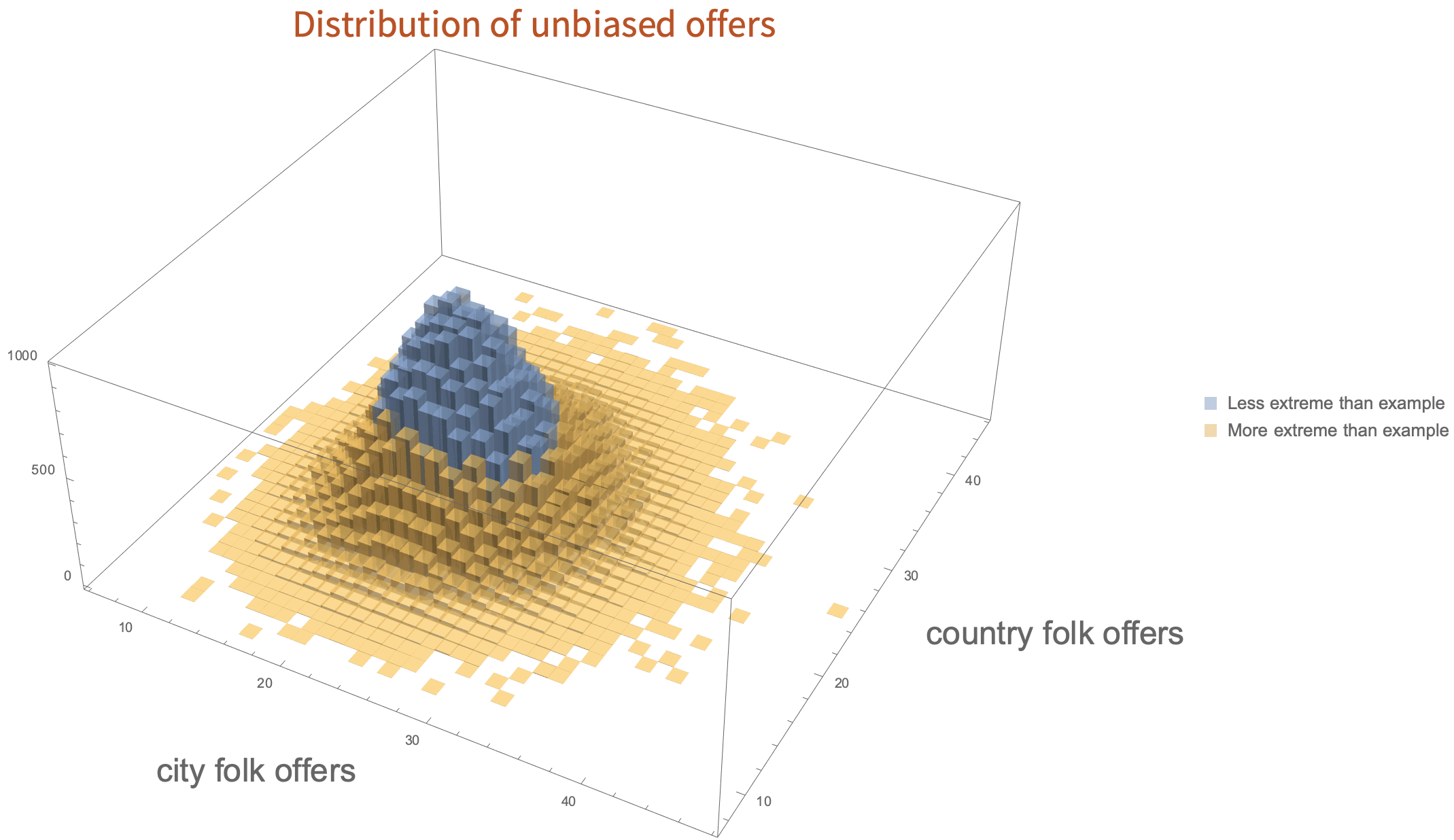
In this figure, everything coloured yellow is at least as far away from fair (22 city offers, 24 country offers) as the example we gave (25 offers out of 100 for city folk and 20 out of 110 for country folk) - even though the algorithm was unbiased. The blue values are those that are closer to fair than the values we gave. In fact, for this simulation you will get results more extreme than those we gave more than half of the time. So, the numbers in the example don’t give strong evidence of bias, because there is a plausible explanation just due to random sampling.

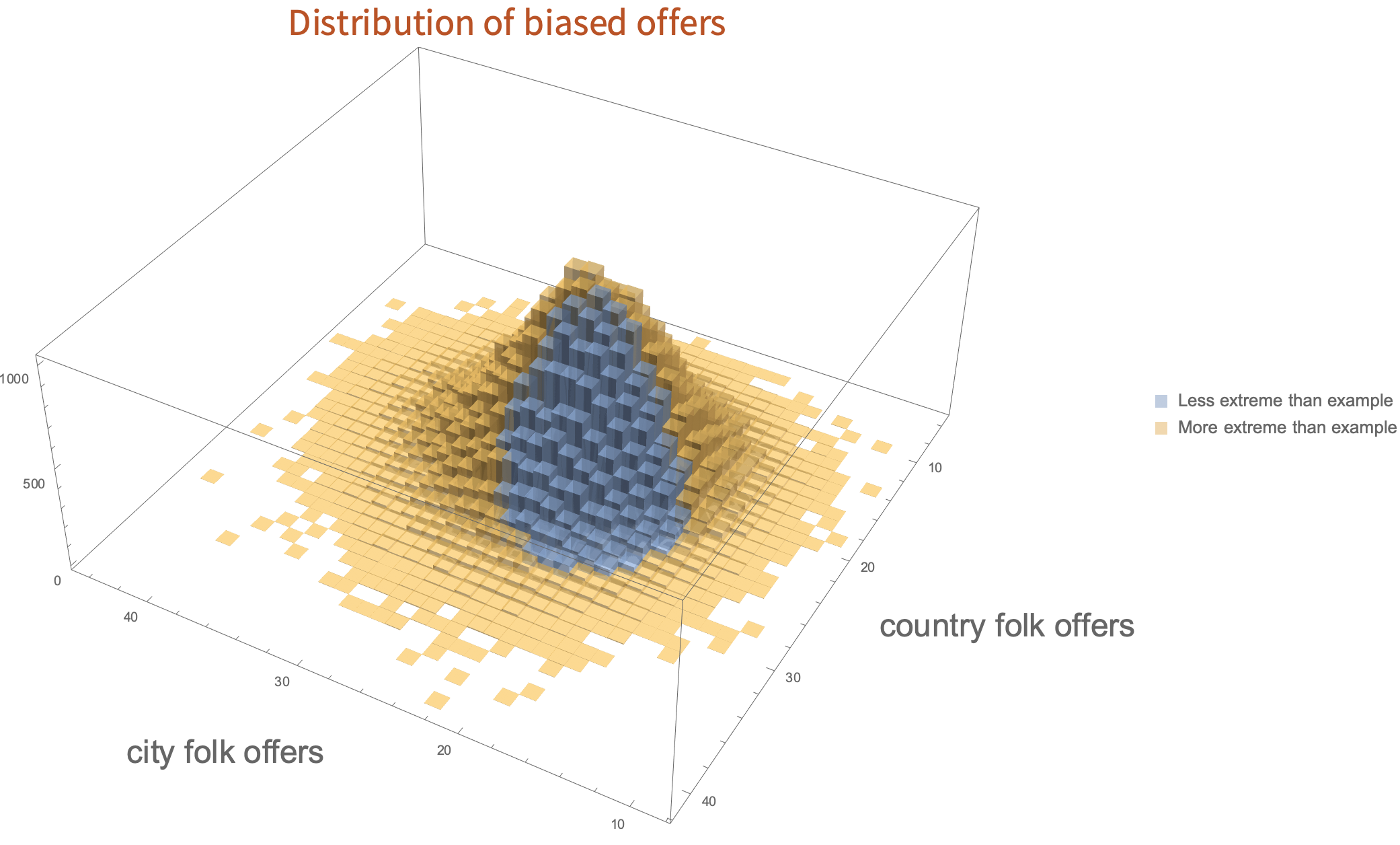
The converse situation can also happen - just say the algorithm was biased and the rates are 18% of country folk get a discount versus 25% of city folk. This case, if we run another simulation, many times the result will look less-biased than the actual bias in the algorithm.

So, given some observations of outcomes, what we need is a clear way of deciding whether there is good evidence that an algorithm is biased or not. Once we have that information, we can decide what to do with it.

More uncertainty

We can view this another way - let us imagine that we have an unbiased algorithm that is deciding to send offers or not. We can plot the observed difference in offers between the two subgroups as the offers are made and compare it to a “fairness threshold” which we sill set to 10%.

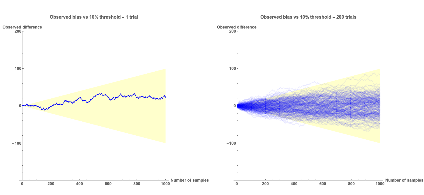
In the plots above we show a single simulation which shows the observed difference in outcomes as a function of the number of offers that have been sent. The yellow region shows the area that is within 10%. The plot on the left shows a single simulation - it shows in this case that the algorithm produces results that look like they are biased less than 10%. The plot on the right shows the traces of 200 such simulations. Clearly, early in the simulation the outcomes look more than 10% biased for a good fraction of the different runs. If we have a bias detection algorithm based on this 10% threshold, we would make a lot of incorrect assessments that the algorithm was biased, when it is not.

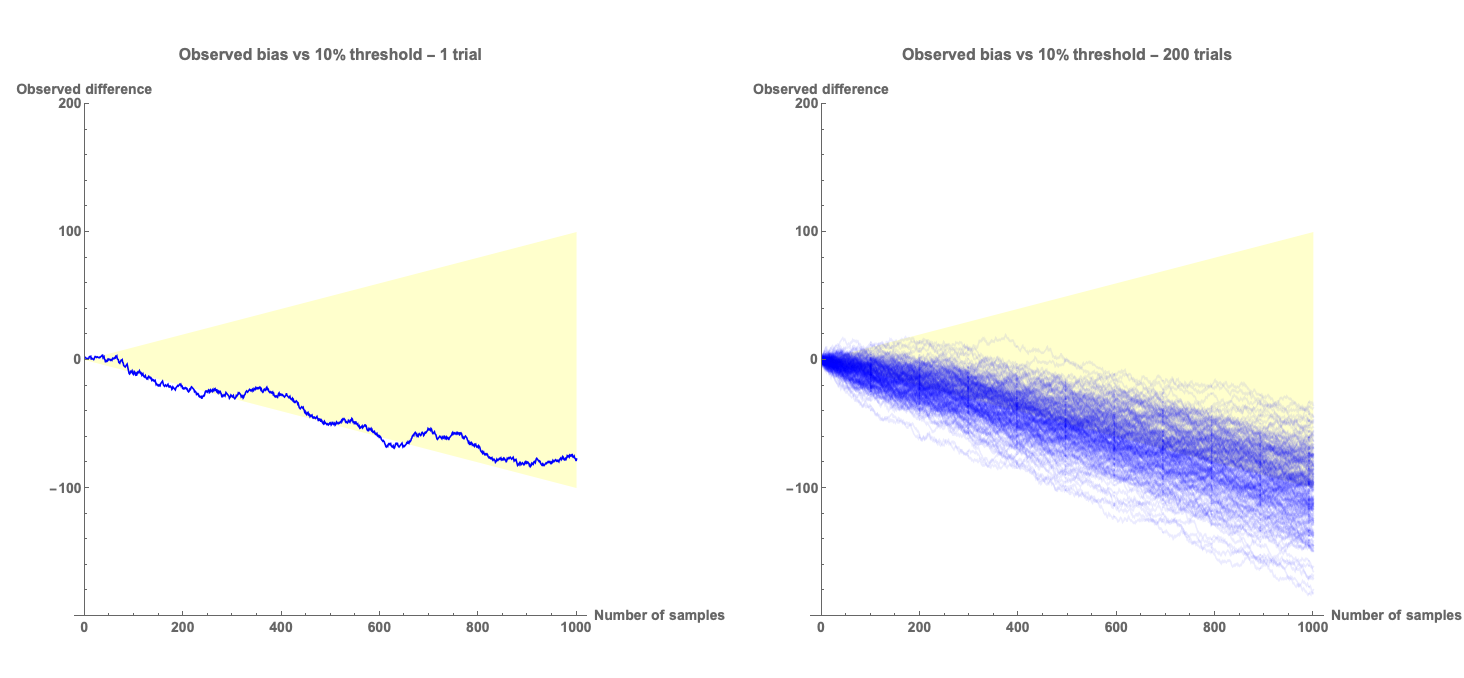
Conversely, the plots above show the situation where there is a 10% bias in the algorithm. In this case there are many cases where, if we made a decision based on the 10% threshold, then we would make a lot of incorrect assessments that the algorithm is not biased, even though it is.

Clearly we need a method of determining whether there is bias that takes into account the sampling errors inherent in the measurement process.

Bias measurement methods for statistical parity

Bias measurement

For a classification algorithm that relates to people (examples are next-best-action recommendation, product recommendation, credit decisioning, etc.), the question we want to answer is whether or not a selection is made by the algorithm at a different rate between one subgroup and another. Let’s say there have been ^n^ classifications made so far - of those ^n_1^ belong to a certain subgroup, and ^n_2^ are not in that subgroup. Of those ^n_1^ people in the subgroup, ^x_1^ received a certain outcome, and of the ^n_2^ people, ^x_2^ received the same outcome. (In our example above - ^n_1=100^, ^x_1=25^, ^n_2=110^, ^x_2=20^).

Taking a Bayesian decision making approach (see below for details), the simplest method to determine whether or not there is a bias is to calculate the expected mean and variance of the difference in rate of outcome selection between group 1, ^r_1^ and group 2, ^r_2^. These are given by

^^\left<r_2-r_1 \right> = \mu \approx -(x_1/n_1) + x_2/n_2^^

and

^^\left<(r_2 - r_1 - \mu)^2 \right> = \sigma^2 \approx \frac{x_1 (n_1-x_1)}{n_1^3}+\frac{x_2 (n_2-x_2)}{n_2^3} ^^

These expressions are approximate - the more accurate formulas are given below.

We’ve seen above that it is possible to make incorrect decisions as to whether or not a set of observations is caused by bias in the algorithm. The question then is: how certain do you want to be? The typical scientific approach would be to consider something like the 68-95-99.7 rule, which specifies how many standard deviations away from the mean you need to be to consider an effect to be significant.

If we set our threshold at 3 standard deviations, then if ^\mu > 0^ and ^\mu - 3 \sigma > 0^ then we have a bias towards group 2 with 99.7 percent confidence.

If ^\mu < 0^ and ^\mu + 3 \sigma < 0^ then we have a bias towards group 1 with 99.7 percent confidence.

Now, different applications of automated decisioning will require different thresholds for bias, and different levels of confidence, based on the impact of the outcomes that are being predicted. This will depend on the impact that false positives (concluding an algorithm is biased when it is not) and false negatives (concluding an algorithm is unbiased when it is not) have on end users, and on how long you can wait for such a result. Given a threshold, ^T^ and a confidence selected by selecting a factor parameterized by a factor ^z^, where 68% (^z=1^), 95% (^z=2^), and 99.7% (^z=3^). We apply the following algorithm:

Simple Algorithm

1. Collect the number of recommendations and total number of people for the subgroups being compared: ^x_1^,^n_1^, ^x_2^, and ^n_2^.
2. Calculate ^\mu^ and ^\sigma^
3. Check if ^\mu - z \sigma > T^ or ^\mu + z \sigma < -T^
4. If either of these conditions is true, then your algorithm is probably operating outside of its acceptable bounds.

Accuracy of measurement

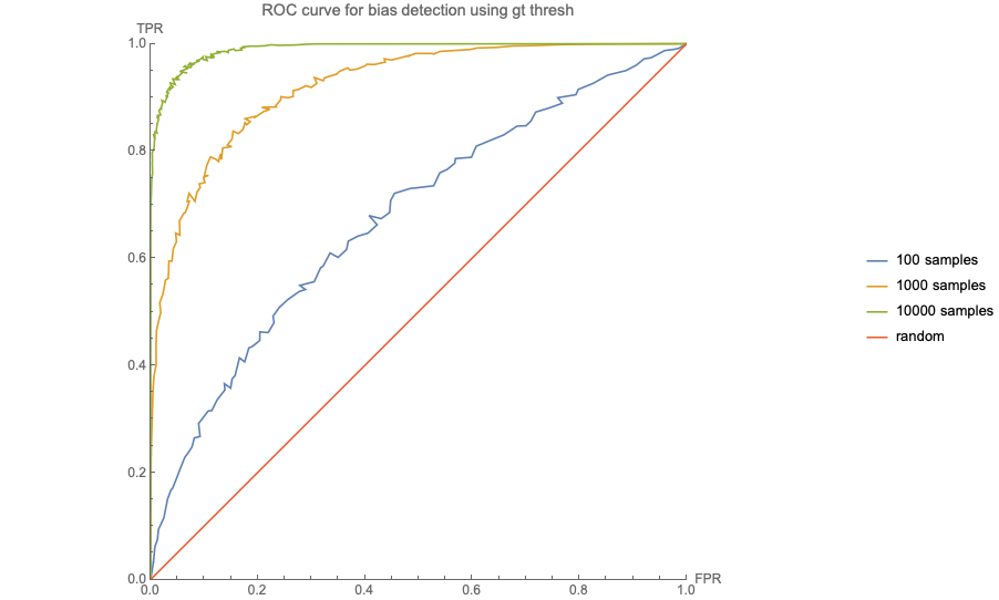
The simple algorithm shown above is essentially a method of deciding whether a set of outcomes shows more bias with respect to statistical parity than the specified threshold. We have seen that it is possible to reach an incorrect conclusion about the presence or absence of bias just because you cannot predict how much noise is in a single observation. It is interesting to ask how often this will happen, and then select our thresholds appropriate to the risk inherent in the use case. To illustrate this, we do a simulation of a biased decision making process and see how often the bias is detected.

We generate sets of ^N^ biased decisions between two subgroups, where the amount of bias is randomly chosen between 0 and 20%. We then see if the algorithm thinks there is more than 10% bias, and compare the answer to the ground truth bias rate as randomly chosen. We do this thousands of times for each confidence threshold and measure the True Positive Rate (the number of times the algorithm said there was more than 10% bias within the specified confidence and there was) and the False Positive Rate (the number of times the algorithm said there was more than 10% bias within the specified confidence and there wasn’t). We plot this below for ^N=100^ samples, ^N=1000^ samples, and ^N=10000^ samples.

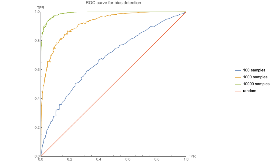
In the plot above, the red line represents an algorithm that is no better than random in detecting bias. As the number of samples increases, the performance of the method improves. For 10,000 samples, represented by the green line, setting the confidence to 90%, less than 1% of unbiased algorithms will be flagged as biased, and more than 80% of biased algorithms will be flagged.

However, if there are only 100 samples, the same settings will flag 5% of unbiased algorithms as biased, and only detect 20% of biased algorithms.

This is very similar to the experimental framework in A/B testing (see our blog post on how we do this), and the warnings and rules about early stopping criteria apply equally well to bias detection in algorithms as they do to experimentation.

Interim Conclusions

If you are just after a simple understanding of the mechanisms for determining if there is bias in your algorithmic results, then you can stop here.

We’ve explained the simple method of detection of biases in deployed automated decisioning systems that we use. You can select a confidence required and a threshold and monitor your algorithms to make sure they don’t go outside these boundaries. Like all experimental methods, this approach must be employed carefully, with a clear understanding of the fact that random noise from sampling can lead to false detections of bias, or fail to detect it when it is present.

We’ve implemented this in our machine learning measurement and experimentation systems, Atmosphere - if you would like to know more,or would like support in measuring and controlling bias in your AI, reach out to us or on the web form on our main page.

Explanation of method

What follows now is a more in-depth analysis of the maths underlying the above, and a comparison of a few other methods that can be used.

Probability distributions

We are interested in the rate of selection of a given outcome by our decision making algorithm for each subgroup, averaged over the population that the algorithm is operating on. We can consider the outcomes as a set of Bernoulli trials, which are modelled by the Binomial distribution. The conjugate distribution to the Binomial distribution is given by the Beta distribution,

^^ p(x,n,e) = \frac{e^x (1-e)^{n-x}}{B(x+1,n-x+1)} ^^

which is an expression for the probability density function of the rate of the underlying process, ^e^, given the observed ^x^ and ^n^.

^^ \int_0^1 p(x,n,e) \, de = 1 ^^. We can illustrate these distributions using some examples. We consider three scenarios:

• We have acted in one way to 20 of one subgroup of 100 people, and in the same way to 30 of another subgroup of 100 people. This case corresponds to it looking like there is a 10% bias in our selection rate.
• We have acted in one way to 40 of one subgroup of 80 people, and in the same way to 20 of another subgroup of 40 people. This case corresponds to it looking like there is no bias in our selection rate.
• We have acted in one way to 400 of one subgroup of 1000 people, and in the same way to 600 of another subgroup of 1000 people. This case corresponds to it looking like there is a 20% bias in our selection rate.

Consider first the joint probability density of the two selection rates.

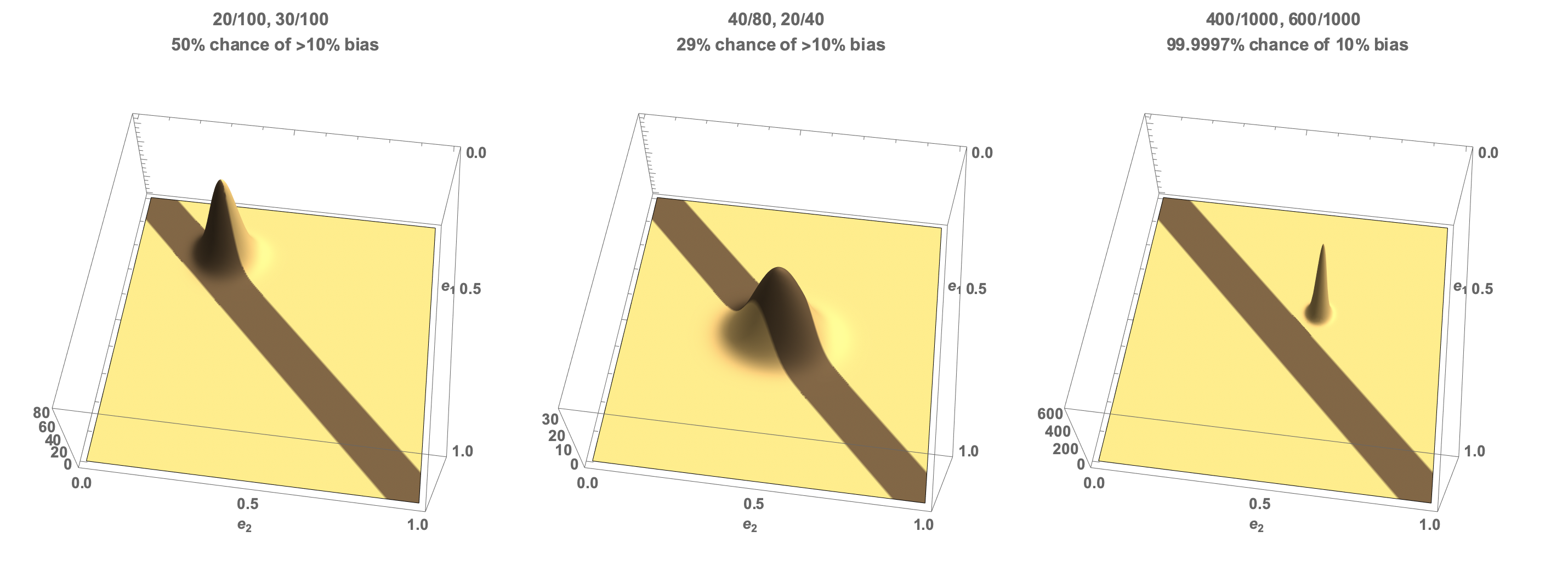
This chart shows the three cases. The x and y axes correspond to the selection rate for each subgroup, and the z axis is the probability density that those selection rates held given the data we have observed. Yellow represents thearea outside our 10% bias threshold, and brown within the 10% bias threshold.

• In case one, the density is peaked at the observed rates of (0.2,0.3). Half of the probability density lies within the 10% threshold and half outside the threshold. So our confidence in at least a 10% bias is exactly 50%.
• In case two, the density is peaked at (0.0,0.0) as the observed rates are equal. However, there is still some probability that the true rates are outside our threshold - 29% of the probability density lies outside our 10% limit, so we have 71% confidence that the underlying selection process is biased less than 10%.
• In case three, the vast majority of the probability density is outside our threshold. So we are very confident (5 nines, in fact) that there is more than 10% bias.

Expected bias

Let’s consider the expected difference in underlying rates given the observed data using these distributions. To do this we multiply the probability density by the difference in rates, which is given by ^e_2 - e_1^ and integrate. Looking at the shapes of these functions is instructive.

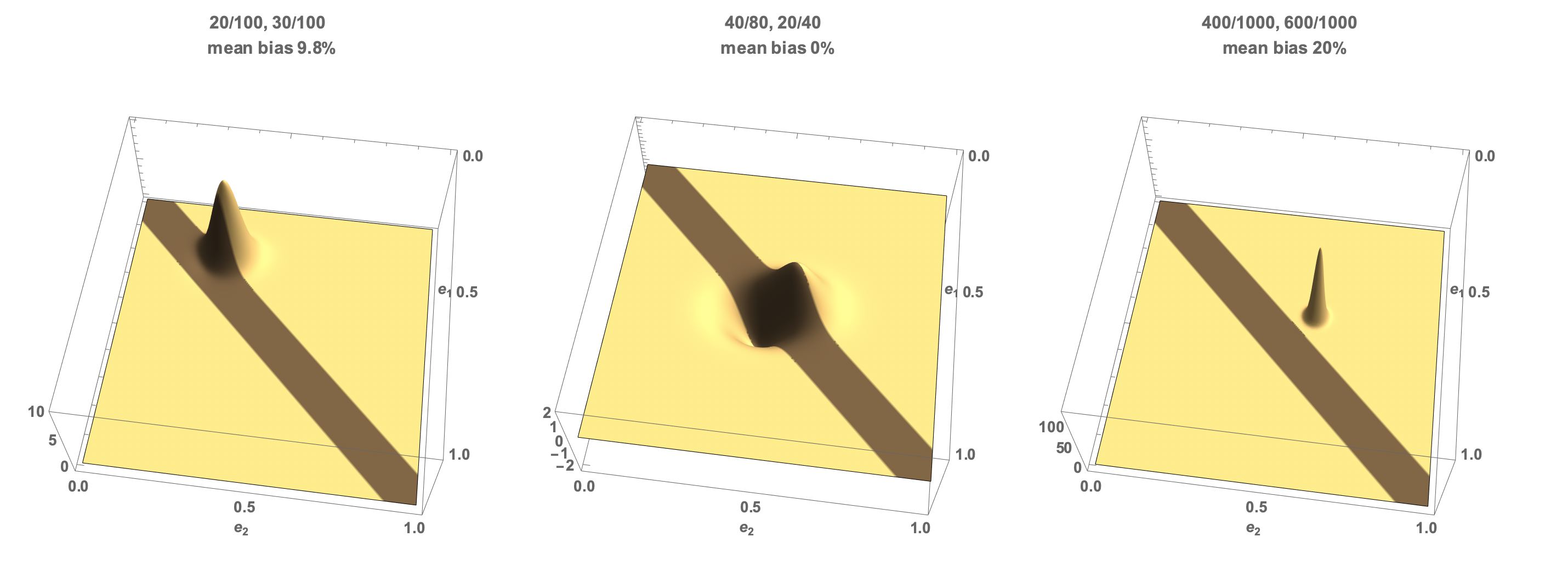
Using the same three cases:

• Here the scaling by the difference in rates leads to an average value of 9.8% bias - there is a small probability mass with support for a bias less than zero which reduces the predicted rate below the observed 10%.
• Here the probability of a negative bias cancels the probability of a positive bias and the expected bias is 0.
• In the third case the mean bias is the same as the observed bias as it is well removed from the zone of uncertainty.

Mathematically speaking, the expected difference in rates given ^x_1^,^n_1^, ^x_2^, and ^n_2^ is given by

^^ \begin{align} \mu = \left< e_2 - e_1\right> & = \int _0^1\int _0^1\left(e_2-e_1\right) p\left(x_1,n_1,e_1\right) p\left(x_2,n_2,e_2\right)\,de_1\,de_2 \\ & = \frac{n_1 x_2-n_2 x_1+n_1-n_2-2 x_1+2 x_2}{\left(n_1+2\right) \left(n_2+2\right)} \\ & \approx \frac{x_2}{n_2} - \frac{x_1}{n_1} \end{align} ^^

Expected variance in bias estimate

The variance is a more complicated calculation, involving weighting the probability distribution by the square of the difference from the mean, ^(e_2 - e_1 - \mu)^2^. This can be plotted in the same way, and the predicted bias is the integral over these distributions.

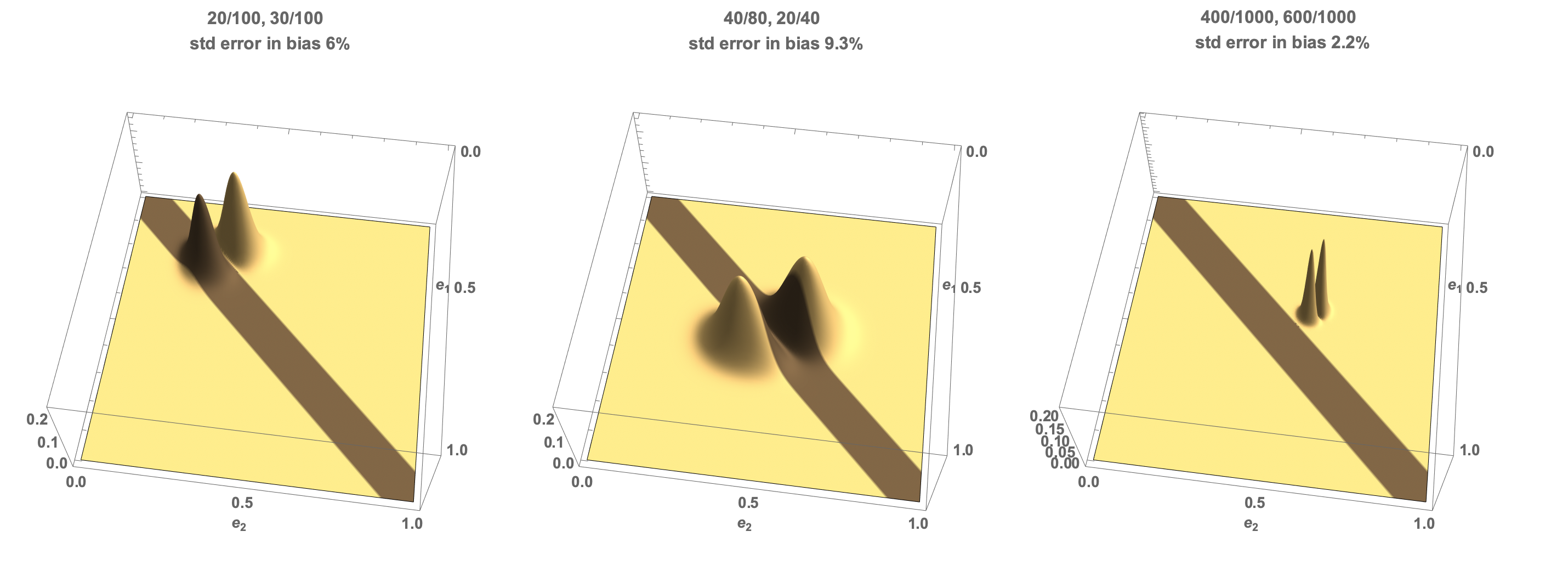
The algebra is more complicated again and given by the following expression, where we have done a power series expansion in quantities scaling as the inverse of the counts.

^^ \begin{align} \sigma^2 = \left< \left(e_2 - e_1 - \mu\right)^2 \right> & = \int _0^1\int _0^1\left(e_2-e_1-\mu \right){}^2 p\left(x_1,n_1,e_1\right) p\left(x_2,n_2,e_2\right)\,de_1\,de_2\\ & = \frac{1}{\left(n_1+2\right)\left(n_1+3\right) \left(n_2+2\right) \left(n_2+3\right)} \times \\ & \left(36 \mu ^2+6 \mu ^2 n_1^2+\mu ^2 n_1^2 n_2^2+5 \mu ^2 n_1 n_2^2+6 \mu ^2 n_2^2+30 \mu ^2 n_1+5 \mu ^2 n_1^2 n_2+ \right.\\ & \left. 25 \mu ^2 n_1 n_2+30 \mu ^2 n_2-6 \mu n_1^2+2 \mu n_1 n_2^2+6 \mu n_2^2-18 \mu n_1-2 \mu n_1^2 n_2+ \right. \\ & \left. 18 \mu n_2+2 \mu n_1 n_2^2 x_1+6 \mu n_2^2 x_1+12 \mu n_1 x_1+10\mu n_1 n_2 x_1+30 \mu n_2 x_1- \right. \\ & \left. 6 \mu n_1^2 x_2-30 \mu n_1 x_2-2 \mu n_1^2 n_2 x_2-10 \mu n_1 n_2 x_2-12 \mu n_2 x_2+n_2^2 x_1^2+ \right. \\ & \left. 5 n_2 x_1^2+n_1^2 x_2^2+5 n_1 x_2^2+3 n_2^2 x_1-6 n_1 x_1-2 n_1 n_2 x_1+9 n_2 x_1+3 n_1^2 x_2+ \right. \\ & \left. 9 n_1 x_2-2 n_1 n_2 x_2-6 n_2 x_2-6 n_1 x_1 x_2-2 n_1 n_2 x_1 x_2-6 n_2 x_1 x_2+2 n_1^2+2 n_2^2+ \right. \\ & \left. 4 n_1-2 n_1 n_2+4 n_2+36 \mu x_1-36 \mu x_2+6 x_1^2+6 x_2^2-18 x_1 x_2+6\right) \\ & \approx \frac{x_1 (n_1-x_1)}{n_1^3}+\frac{x_2 (n_2-x_2)}{n_2^3} \end{align} ^^

The mean and variance can be calculated using the following C code - note that this calculates the variance - the standard deviation is the square root of this.

m = (n1 - n2 - 2*x1 - n2*x1 + 2*x2 + n1*x2)/((2 + n1)*(2 + n2));
ms = m*m;
n1s = n1*n1;
n2s = n2*n2;
x1s = x1*x1;
x2s = x2*x2;
var = (6 + 36*ms + 4*n1 - 18*m*n1 + 30*ms*n1 + 2*n1s - 6*m*n1s + 6*ms*n1s + 4*n2 + 18*m*n2 + 
   30*ms*n2 - 2*n1*n2 + 25*ms*n1*n2 - 2*m*n1s*n2 + 5*ms*n1s*n2 + 2*n2s + 6*m*n2s + 
   6*ms*n2s + 2*m*n1*n2s + 5*ms*n1*n2s + ms*n1s*n2s + 36*m*x1 - 6*n1*x1 + 
   12*m*n1*x1 + 9*n2*x1 + 30*m*n2*x1 - 2*n1*n2*x1 + 10*m*n1*n2*x1 + 3*n2s*x1 + 6*m*n2s*x1 + 2*m*n1*n2s*x1 + 
   6*x1s + 5*n2*x1s + n2s*x1s - 36*m*x2 + 9*n1*x2 - 30*m*n1*x2 + 3*n1s*x2 - 6*m*n1s*x2 - 6*n2*x2 - 
   12*m*n2*x2 - 2*n1*n2*x2 - 10*m*n1*n2*x2 - 2*m*n1s*n2*x2 - 18*x1*x2 - 6*n1*x1*x2 - 6*n2*x1*x2 - 2*n1*n2*x1*x2 + 6*x2s + 
   5*n1*x2s + n1s*x2s)/((2 + n1)*(3 + n1)*(2 + n2)*(3 + n2));

Comparisons

There are other methods of measuring bias, also based on Bayesian approaches, that rely on the distribution of the differences of the rate variables. If we define a random variable ^T = X_2 - X_1^, where ^X_1^ and ^X_2^ are distributed according to the Beta distribution used above, then the cumulative distribution function of ^T^ is given by the convolution of the distributions of ^X_1^ and ^X_2^, and the variate, ^\tau^ ranges from -1 to 1.

^^ \begin{align} P(T>\tau|x_1,n_1,x_2,n_2) = & \frac{B_{\min (1,1+\tau )}(1+x_1,1+n_1-x_1)}{B(1+x_1,1+n_1-x_1)}-\\ &\int_{\max (0,\tau )}^{\min (1,1+\tau )} \frac{\left((1-e_1)^{n_1-x_1} e_1^{x_1}\right) (B_{e_1-\tau }(1+x_2,1+n_2-x_2) \Gamma (2+n_2))}{B(1+x_1,1+n_1-x_1) (\Gamma (1+n_2-x_2) \Gamma (1+x_2))} \, de_1 \end{align} ^^ where ^B_z(a,b)^ and ^B(a,b)^ are the incomplete Beta function and the Beta function respectively. This CDF has no closed form solution, however it can be evaluated readily using numerical integration packages.

Using this CDF, an alternative algorithm can be developed. Given a threshold, ^t^ and a confidence ^c^:

Algorithm 2 - probability of deviation

1. Collect the number of recommendations and total number of people for the subgroups being compared: ^x_1^,^n_1^, ^x_2^, and ^n_2^.
2. Calculate p = P(T>t) + P(T<-t)
3. Check if p > c
4. If this condition is true, your algorithm is probably operating outside its acceptable bounds.

Note that this is equivalent to using a step-function ^H(e_2-e_1)^ to weight the probability density rather than the difference in rates as used in the method presented above.

We can evaluate this approach using the same simulations as performed in the main method. In this case, the execution time is much more than 10 times slower than the method based on the expected rate difference presented above. The performance in terms of the ROC curve is essentially indistinguishable

The probability density function for ^T^ is given by the derivative of the CDF with respect to ^\tau^. It is included here for reference: ^^ P(\tau|x_1,n_1,x_2,n_2) = \int_{\max (0,\tau )}^{\min (1,1+\tau )} \frac{\left((1-e_1)^{n_1-x_1} e_1^{x_1}\right) \left((e_1-\tau )^{x_2} (1-e_1+\tau )^{n_2-x_2}\right)}{B(1+x_1,1+n_1-x_1) B(1+x_2,1+n_2-x_2)} \, de_1 ^^

The probability density function can be used to calculate the High Density Interval (HDI) - a range of values which contain a certain proportion of the probability density. The HDI is illustrated in the figure below, for the confidence levels equivalent to 1 sigma, 2 sigma and 3 sigma errors.

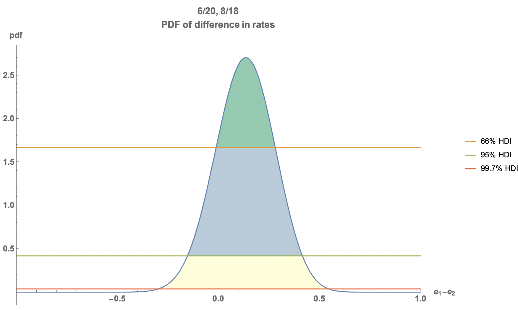
This plot shows that for the parameters given, we can determine a range of bias values for which we have confidence above a certain threshold. More detail around the HDI is covered in our experimentation blog post. The HDI can be used to decide if there is significant bias in an algorithm. Again, as an input the user selects a confidence threshold, ^c^, and a level at which they would consider the bias significant, ^t^ (or Region Of Practical Equivalence (ROPE)).

Algorithm 3

1. Collect the number of recommendations and total number of people for the subgroups being compared: ^x_1^,^n_1^, ^x_2^, and ^n_2^.
2. Calculate the bounds of the HDI: (lower,upper) = HDI(c)
3. Check if the HDI intersects the range (-t,t), i.e. if upper > -t or lower < t.
4. If this condition is true, your algorithm is probably operating outside its acceptable bounds.

The HDI+ROPE test is an elegant solution to the detection of bias in an algorithm, but is significantly slower than the other methods, as it requires the detection of the HDI interval for each test, where the evaluation of the PDF above requires a complex (and sometimes unstable) numerical integral.

To illustrate this method of determining whether bias is present using the HDI, consider the following plots, which use the same illustrative parameters as before.

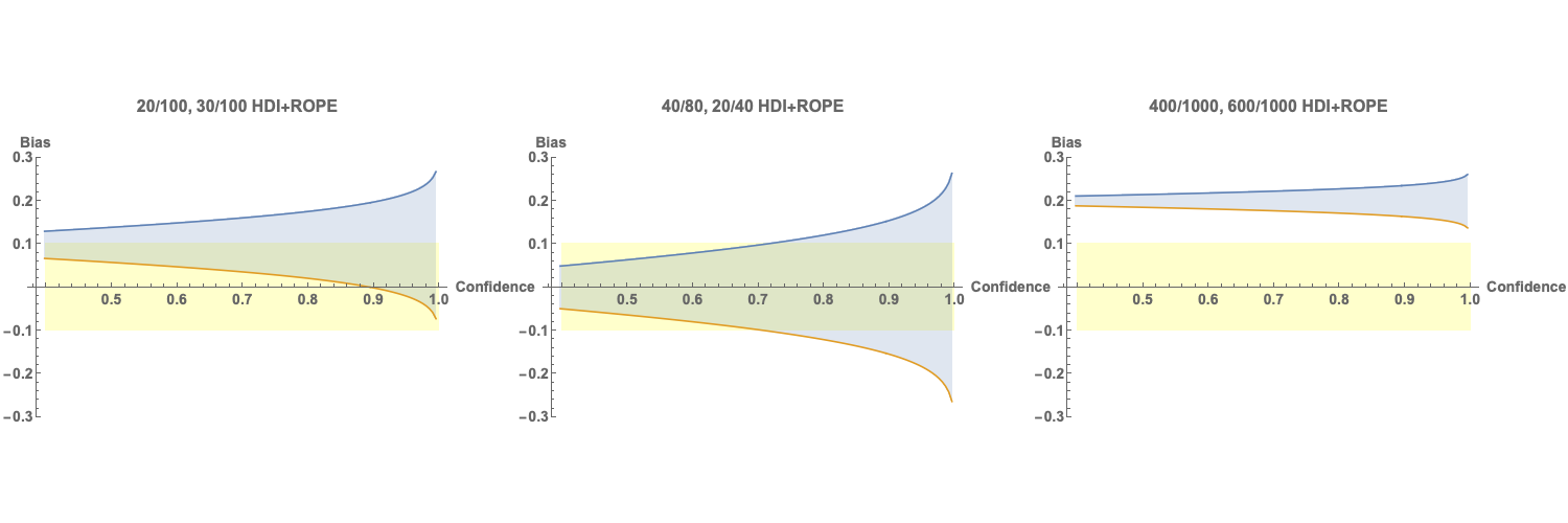
In this figure, we plot the upper and lower bounds of the HDI for the bias as a function of the confidence we have in the presence of bias. So, at 50% confidence, we can expect the bias to be within a certain range. As we increase our confidence the range of values covered increases - as we have to consider a wider range of possible values that agree with the data to have higher confidence. The orange line represents the bottom of the range and the blue the top of the range. The yellow bar represents the ROPE - in our example we are investigating whether the bias exceeds 10% - which we can set as our range.

• In the first plot we see that we cannot be sure that the bias exceeds 10% at any confidence level, and can also see that we can’t exclude there being no bias at all at more than 90% confidence (as the orange line drops below 0 at 90%)
• In the second plot we can see that we cannot be sure there is any bias.
• In the third plot, we can be confident at least to the 99% level (to 99.997% in fact) that there is a bias greater than 10%.

The HDI + ROPE method is a great illustrative diagnostic to understand the limits of the data that has been collected.

Learn More

Do you want some help in evaluating your algorithms for bias, detecting bias in production algorithms, or building unbiased algorithms in the first place? If so, Ambiata provides consulting on all of these issues. Contact us at info@ambiata.com or on the web form on our main page.