
Fairness and understanding hidden biases in algorithms used for decision making are increasingly important. In this post, we’ll use open source tools to detect and mitigate algorithmic bias in an example dataset.
Introduction
The field of algorithmic fairness has grown in recent years, and there have been a range of tools developed to measure and control the unintended bias in models, under various definitions of fairness. One of these is the AI Fairness 360 Open Source Toolkit, which is a python module for studying bias in machine learning. It comes with some user-friendly web demos and tutorials, and has been developed with an emphasis on practical application outside of the academic community.
We will use it here in our example problem: a government jobs department tasked with predicting which applicants are likely to get a job.
We begin by loading the packages we’ll be using, including aif360.
import pandas as pd
import numpy as np
import seaborn as sns
import matplotlib.pyplot as plt
from aif360.datasets import BinaryLabelDataset
from aif360.metrics import BinaryLabelDatasetMetric
from aif360.metrics import ClassificationMetric
from aif360.algorithms.preprocessing import Reweighing
from sklearn.preprocessing import StandardScaler
from sklearn.linear_model import LogisticRegression
from tqdm import tqdm
np.random.seed(1)
We also define some functions that will be useful in the following analysis.
def get_disparity_index(di):
    return 1 - np.minimum(di, 1 / di)


def get_bal_acc(classified_metric):
    return 0.5 * (classified_metric.true_positive_rate() + classified_metric.true_negative_rate())


def train_lr_model(dataset):
    scale = StandardScaler().fit(dataset.features)
    model = LogisticRegression(random_state=0, solver='liblinear')
    x_train = scale.transform(dataset.features)
    y_train = dataset.labels.ravel()
    model.fit(x_train, y_train, sample_weight=dataset.instance_weights)
    y_train_pred = model.predict(x_train)
    return model, scale


def test_lr_model(y_data_pred_prob, dataset, thresh_arr):
    y_pred = (y_data_pred_prob[:,1] > thresh_arr).astype(np.double)
    dataset_pred = dataset.copy()
    dataset_pred.labels = y_pred
    classified_metric = ClassificationMetric(dataset, dataset_pred, unprivileged_group, privileged_group)
    metric_pred = BinaryLabelDatasetMetric(dataset_pred, unprivileged_group, privileged_group)
    return dataset_pred.labels, classified_metric, metric_pred


def get_y_pred_prob_lr(scale, model, dataset):
    x = scale.transform(dataset.features)
    y_pred_prob = model.predict_proba(x)
    return y_pred_prob


def get_best_bal_acc_cutoff(y_pred_prob, dataset):
    y_validate_pred_prob = y_pred_prob
    bal_acc_arr = []
    disp_imp_arr = []

    for thresh in tqdm(thresh_arr):
        y_validate_pred = (y_validate_pred_prob[:,1] > thresh).astype(np.double)
        dataset_pred = dataset.copy()
        dataset_pred.labels = y_validate_pred

        # Calculate accuracy for each threshold value
        classified_metric = ClassificationMetric(dataset, dataset_pred, unprivileged_group, privileged_group)
        bal_acc = get_bal_acc(classified_metric)
        bal_acc_arr.append(bal_acc)

        # Calculate fairness for each threshold value
        metric_pred = BinaryLabelDatasetMetric(dataset_pred, unprivileged_group, privileged_group)
        disp_imp_arr.append(metric_pred.disparate_impact())

    # Find threshold for best accuracy
    thresh_arr_best_ind = np.where(bal_acc_arr == np.max(bal_acc_arr))[0][0]
    thresh_arr_best = np.array(thresh_arr)[thresh_arr_best_ind]

    # Calculate accuracy and fairness at this threshold
    best_bal_acc = bal_acc_arr[thresh_arr_best_ind]
    disp_imp_at_best_bal_acc = disp_imp_arr[thresh_arr_best_ind]

    # Output metrics
    acc_metrics = pd.DataFrame({'thresh_arr_best_ind' : thresh_arr_best_ind, \
    'thresh_arr_best' : thresh_arr_best, \
    'best_bal_acc' : best_bal_acc, \
    'disp_imp_at_best_bal_acc' : disp_imp_at_best_bal_acc}, index=[0]).transpose()
    return acc_metrics, bal_acc_arr, disp_imp_arr, dataset_pred.labels


def plot_acc_vs_fairness(metric, metric_name, bal_acc_arr, thresh_arr_best_ind):
    fig, ax1 = plt.subplots(figsize=(10, 7))
    ax1.plot(thresh_arr, bal_acc_arr, color='b')
    ax1.set_xlabel('Classification Thresholds', fontsize=16, fontweight='bold')
    ax1.set_ylabel('Balanced Accuracy', color='b', fontsize=16, fontweight='bold')
    ax1.xaxis.set_tick_params(labelsize=14)
    ax1.yaxis.set_tick_params(labelsize=14, labelcolor='b')
    ax2 = ax1.twinx()
    ax2.plot(thresh_arr, metric, color='r')
    ax2.set_ylabel(metric_name, color='r', fontsize=16, fontweight='bold')
    ax2.axvline(np.array(thresh_arr)[thresh_arr_best_ind], color='k', linestyle=':')
    ax2.yaxis.set_tick_params(labelsize=14, labelcolor='r')
    ax2.grid(True)
Data preparation
Generate the jobseeker population
We will generate a synthetic dataset for this problem. Suppose we are a government unemployment department with population of 100,000 jobseekers, with a 70:30 gender split between males and females. The probability of finding a job after 3 months is 9%, while it is only 5% for females.
n_pop = 100000
p_male = 0.7

p_job_male, p_job_female = 0.09, 0.05
gender = np.random.choice(['male', 'female'], size=n_pop, p=[p_male, 1 - p_male])

df = pd.DataFrame({'gender' : gender})

df.loc[df.gender == 'male', 'found_job'] = np.random.choice([1, 0], size=len(df.loc[df.gender == 'male']), p=[p_job_male, 1 - p_job_male])
df.loc[df.gender == 'female', 'found_job'] = np.random.choice([1, 0], size=len(df.loc[df.gender == 'female']), p=[p_job_female, 1 - p_job_female])

df['found_job'] = df['found_job'].astype(int)
The gender breakdown of jobseekers who find a job or don’t find a job looks like this:
df.pivot_table(index='gender', columns='found_job', aggfunc='size')
.dataframe tbody tr th {
    vertical-align: top;
}

.dataframe thead th {
    text-align: right;
}
We can also assign ages to each jobseeker by sampling from a Gaussian distribution with a mean of mu and a standard deviation of sigma. We will sample from two Gaussian distributions: one for jobseekers who find a job, and one for jobseekers who do not find a job. The age distributions for jobseekers who find a job has a lower mean, this is to reflect the fact that it is easier for younger jobseekers to find work.
mu_job, sigma_job = 45, 8
mu_no_job, sigma_no_job = 55, 10
df.loc[df.found_job == 1, 'age'] = np.floor(np.random.normal(mu_job, sigma_job, len(df.loc[df.found_job == 1])))
df.loc[df.found_job == 0, 'age'] = np.floor(np.random.normal(mu_no_job, sigma_no_job, len(df.loc[df.found_job == 0])))

df['age'] = df['age'].astype(int)
The mean age of jobseekers who find a job or don’t find a job looks like this:
df.groupby('found_job').mean().round(1)
.dataframe tbody tr th {
    vertical-align: top;
}

.dataframe thead th {
    text-align: right;
}
The final attribute we will create for this population is their socioeconomic class, which we will label as A, B, or C, to refer to high, middle, and lower classes, respectively. As with the age distribution, we can sample from two distributions: one for jobseekers who find a job, and one for jobseekers who don’t find a job. The distributions weights are such that jobseekers who find a job tend to belong to higher socioeconomic classes, while jobseekers who don’t find a job tend to come from lower socioeconomic classes.
class_set = ['A', 'B', 'C']
class_wt_job = [0.4, 0.4, 0.2]
class_wt_no_job = [0.2, 0.3, 0.5]
df.loc[df.found_job == 1, 'class'] = np.random.choice(class_set, size=len(df.loc[df.found_job == 1]), p=class_wt_job)
df.loc[df.found_job == 0, 'class'] = np.random.choice(class_set, size=len(df.loc[df.found_job == 0]), p=class_wt_no_job)
The class breakdown of jobseekers who find a job or don’t find a job looks like this:
df.pivot_table(index='class', columns='found_job', aggfunc='size')
.dataframe tbody tr th {
    vertical-align: top;
}

.dataframe thead th {
    text-align: right;
}
Plot the gender bias
Here, we verify that the gender bias with respect to jobseeker success rates agrees with what we initially set.
agg_gender = df[['gender', 'found_job']].groupby('gender').mean()
agg_gender.round(3)
.dataframe tbody tr th {
    vertical-align: top;
}

.dataframe thead th {
    text-align: right;
}
We can also plot the gender bias as follows:
mean_found_job = df['found_job'].mean()

fig, ax1 = plt.subplots(figsize=(10, 7))
sns.barplot(x=agg_gender.index, y=agg_gender.found_job, ax=ax1).\
set_title('Proportion of total who find a job', fontsize=16, fontweight='bold')
ax1.axhline(mean_found_job, color='k', linestyle=':')
ax1.set(xlabel='', ylabel='')
ax1.xaxis.set_tick_params(labelsize=14)
ax1.yaxis.set_tick_params(labelsize=14)
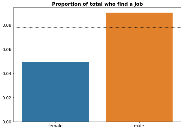
where the dashed line corresponds to the overall probability of finding a job, which is:
print(mean_found_job.round(3))
0.078
Males have a better than average probability to find a job, while females have a lower than average probability to find a job.
Convert to AIF360 format
Now that we have our synthetic jobseeker population, we can convert it into the aif360 format. Firstly, we one-hot encode the gender and class variables.
df_onehot = pd.concat([df[['found_job', 'age']], pd.get_dummies(df[['gender', 'class']])], axis=1)
In our example, the label is binary (they either find a job, or they don’t), so we convert the data into a BinaryLabelDataset, where the binary label is found_job, and the protected attribute is gender_female. We also drop the redundant gender_male column.
df_aif = BinaryLabelDataset(df=df_onehot.drop('gender_male', axis=1), label_names=['found_job'], protected_attribute_names=['gender_female'])
In this situation, the privileged and unprivileged groups are males and females, respectively.
privileged_group = [{'gender_female': 0}]
unprivileged_group = [{'gender_female': 1}]
For modelling purposes, we partition our data in to training, validation, and test datasets.
df_orig_trn, df_orig_val, df_orig_tst = df_aif.split([0.5, 0.8], shuffle=True)
print([x.features.shape for x in [df_orig_trn, df_orig_val, df_orig_tst]])
[(50000, 5), (30000, 5), (20000, 5)]
Original dataset
Now suppose that this government unemployment department wants to allocate more resources to jobseekers who are more likely to find a job, rather than waste them on jobseekers who are less likely to find a job. A predictive model would allow them to identify the two groups of jobseekers automatically.
For the first piece of analysis, we will train a such a model, using the original dataset with its inherent gender bias.
Compute fairness metric on original dataset
There are various fairness metrics available in aif360, but the one we will focus on is the Disparate Impact (DI). This is the probability of success given the jobseeker is unprivileged (female), divided by the probability of success given the jobseeker is privileged (male). We further recast this as 1 - min(DI, 1/DI), since DI can be greater than 1, which would mean that the privileged group is disadvantaged. For our fairness benchmark, we require that 1 - min(DI, 1/DI) < 0.2.
metric_orig_trn = BinaryLabelDatasetMetric(df_orig_trn, unprivileged_group, privileged_group)
print('1-min(DI, 1/DI):', get_disparity_index(metric_orig_trn.disparate_impact()).round(3))
1-min(DI, 1/DI): 0.448
This value of 1 - min(DI, 1/DI) confirms that the original dataset is biased.
Train model on original dataset
Here, we train a logistic regression model on the original training dataset.
lr_orig, lr_scale_orig = train_lr_model(df_orig_trn)
Find cutoff threshold using original validation dataset
We now use the model to score the original validation dataset, and calculate the balanced accuracy using various cutoff thresholds. The threshold with the best balanced accuracy will be the one we use.
thresh_arr = np.linspace(0.01, 0.5, 100)
y_validate_pred_prob_orig = get_y_pred_prob_lr(scale=lr_scale_orig, model=lr_orig, dataset=df_orig_val)
acc_metrics_orig, bal_acc_arr_orig, disp_imp_arr_orig, dataset_pred_labels_orig = \
get_best_bal_acc_cutoff(y_pred_prob=y_validate_pred_prob_orig, dataset=df_orig_val)
100%|██████████| 100/100 [00:02<00:00, 37.39it/s]
print('Threshold corresponding to best balanced accuracy:', acc_metrics_orig.loc['thresh_arr_best', 0].round(3))
print('Best balanced accuracy:', acc_metrics_orig.loc['best_bal_acc', 0].round(3))
print('1-min(DI, 1/DI):', get_disparity_index(acc_metrics_orig.loc['disp_imp_at_best_bal_acc', 0]).round(3))
Threshold corresponding to best balanced accuracy: 0.074
Best balanced accuracy: 0.759
1-min(DI, 1/DI): 0.459
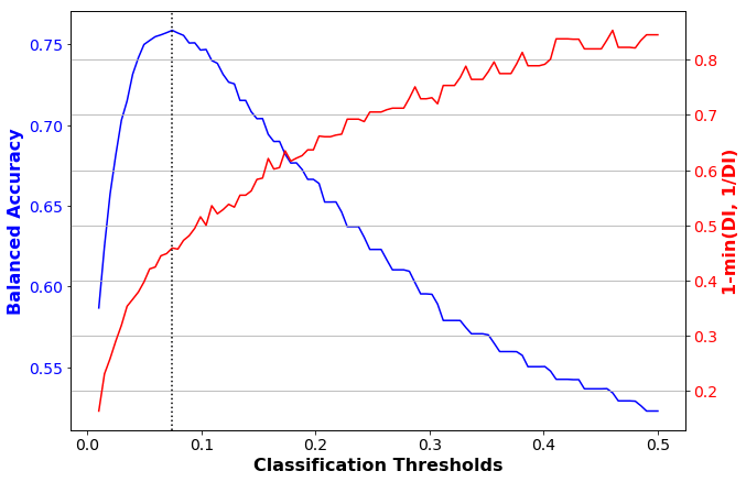
This shows that the threshold with the best accuracy is 0.074. At this threshold, our accuracy metric (balanced accuracy) is 0.759, but our fairness metric (1-min(DI, 1/DI)) is 0.459, which indicates bias. We can plot these accuracy and fairness metrics over a range of classification thresholds:
plot_acc_vs_fairness(get_disparity_index(np.array(disp_imp_arr_orig)), \
  '1-min(DI, 1/DI)', bal_acc_arr_orig, \
  acc_metrics_orig.loc['thresh_arr_best_ind', 0].astype(int))
Test model on original dataset
We can now take the model and the cutoff threshold to score the original holdout test dataset.
y_test_pred_prob_orig = get_y_pred_prob_lr(scale=lr_scale_orig, model=lr_orig, dataset=df_orig_tst)

dataset_pred_labels_orig, classified_metric_orig, metric_pred_orig = test_lr_model(\
  y_data_pred_prob=y_test_pred_prob_orig, dataset=df_orig_tst,\
  thresh_arr=acc_metrics_orig.loc['thresh_arr_best', 0])
print('Threshold corresponding to best balanced accuracy:', acc_metrics_orig.loc['thresh_arr_best', 0].round(3))
print('Best balanced accuracy:', get_bal_acc(classified_metric_orig).round(3))
print('1-min(DI, 1/DI):', get_disparity_index(metric_pred_orig.disparate_impact()).round(3))
Threshold corresponding to best balanced accuracy: 0.074
Best balanced accuracy: 0.75
1-min(DI, 1/DI): 0.466
As with the validation dataset, we end up with a good accuracy metric, but a poor fairness metric. This shows that if we only consider accuracy (as is common in many organisations), we end up with a model that is unfair.
Bias mitigation
To mitigate the effects of the gender bias in our original dataset, we can transform the dataset using a pre-processing technique called reweighing. This assigns different weights to the various entities in the population to ensure fairness.
RW = Reweighing(unprivileged_group, privileged_group)
df_transf_trn = RW.fit_transform(df_orig_trn)
Compute fairness metric on transformed dataset
When we compute the fairness metric on the transformed dataset, we see that it is fair.
metric_transf_trn = BinaryLabelDatasetMetric(df_transf_trn, unprivileged_group, privileged_group)
print('1-min(DI, 1/DI):', get_disparity_index(metric_transf_trn.disparate_impact()).round(3))
1-min(DI, 1/DI): 0.0
Train model on transformed dataset
Now that we have the transformed dataset, we can train a model on it as we did before. This new model will be fairer than the previous one.
lr_transf, lr_scale_transf = train_lr_model(df_transf_trn)
Find cutoff threshold using transformed validation dataset
We use the new, fairer model to score the original validation dataset, and find the cutoff threshold with the best balanced accuracy.
y_validate_pred_prob_transf = get_y_pred_prob_lr(scale=lr_scale_transf, model=lr_transf, dataset=df_orig_val)
acc_metrics_transf, bal_acc_arr_transf, disp_imp_arr_transf, dataset_pred_labels_transf = \
get_best_bal_acc_cutoff(y_pred_prob=y_validate_pred_prob_transf, dataset=df_orig_val)
100%|██████████| 100/100 [00:02<00:00, 36.19it/s]
print('Threshold corresponding to best balanced accuracy:', acc_metrics_transf.loc['thresh_arr_best', 0].round(3))
print('Best balanced accuracy:', acc_metrics_transf.loc['best_bal_acc', 0].round(3))
print('1-min(DI, 1/DI):', get_disparity_index(acc_metrics_transf.loc['disp_imp_at_best_bal_acc', 0]).round(3))
Threshold corresponding to best balanced accuracy: 0.074
Best balanced accuracy: 0.753
1-min(DI, 1/DI): 0.062
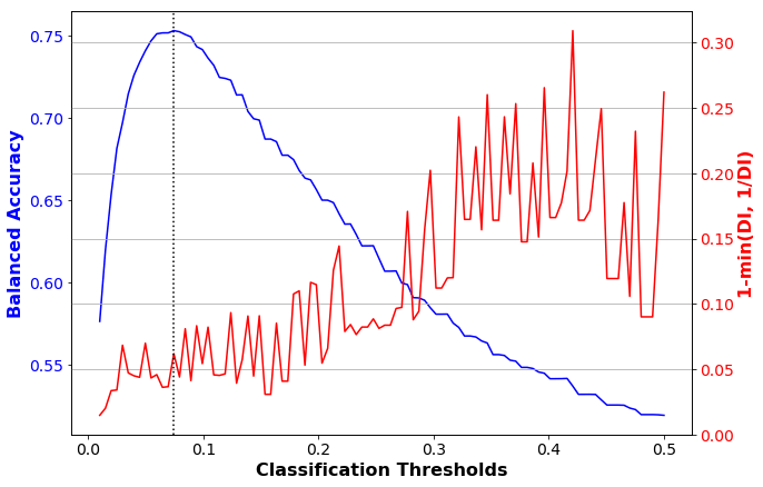
This shows that the threshold with the best accuracy is still 0.074. At this threshold, our accuracy metric (balanced accuracy) is 0.753, and our fairness metric (1-min(DI, 1/DI)) is 0.062, which indicates no bias. We can plot these accuracy and fairness metrics over a range of classification thresholds:
plot_acc_vs_fairness(get_disparity_index(np.array(disp_imp_arr_transf)), \
  '1-min(DI, 1/DI)', bal_acc_arr_transf, \
  acc_metrics_orig.loc['thresh_arr_best_ind', 0].astype(int))
Test model on transformed dataset
We can now take the fairer model and the cutoff threshold to score the original holdout test dataset.
y_test_pred_prob_transf = get_y_pred_prob_lr(scale=lr_scale_transf, model=lr_transf, dataset=df_orig_tst)

dataset_pred_labels_transf, classified_metric_transf, metric_pred_transf = test_lr_model(\
  y_data_pred_prob=y_test_pred_prob_transf, dataset=df_orig_tst,\
  thresh_arr=acc_metrics_transf.loc['thresh_arr_best', 0])
print('Threshold corresponding to best balanced accuracy:', acc_metrics_transf.loc['thresh_arr_best', 0].round(3))
print('Best balanced accuracy:', get_bal_acc(classified_metric_transf).round(3))
print('1-min(DI, 1/DI):', get_disparity_index(metric_pred_transf.disparate_impact()).round(3))
Threshold corresponding to best balanced accuracy: 0.074
Best balanced accuracy: 0.742
1-min(DI, 1/DI): 0.068
As with the validation dataset, we end up with a good accuracy and fairness metrics. The bias mitigation has caused the accuracy to slightly worsen (from 0.75 to 0.742), but the fairness to greatly improve (0.466 to 0.068). This shows that models that are both accurate and fair can be built on biased data, as long as bias mitigation is applied appropriately.
Conclusion
We have seen here how a dataset with historical bias will cause models built on it to produce unfair results. In our scenario, more resources would be allocated to males, because they have historically been more likely to find a job. This is because traditional machine learning techniques optimise for accuracy only, not fairness. We have also seen that by applying simple bias mitigation techniques, we can remove the bias from the dataset and thus create models with comparable accuracy, but much better fairness metrics. These bias detection and mitigation techniques are highly relevant for any organisation seeking to automate decision making on populations with protected attributes.
Photo credit: unsplash-logoBill Oxford