
The ability to test decision-making algorithms without actually deploying them to live systems is an important feature for automated decision-making systems to have. In this post, we examine how this testing can be done on real data, to ensure that algorithms are properly vetted before deployment.
Decision-making algorithms (e.g. contextual bandit algorithms [1]) are designed to interact with the real world in an automated way. However, care must be taken in how these algorithms are deployed, because their automated nature means that errors can lead to runaway algorithms, with adverse consequences. We would like to have the ability to evaluate how an algorithm will perform, without the risk of deploying a poorly performing algorithm to a production system. The ability to rapidly iterate such a process would also help optimise the algorithm, as different parameters could be tuned quickly without the risk of harm to the production system.
While the most accurate demonstration of how an automated algorithm will perform is to actually deploy it, there are often circumstances where this is impractical. An alternative approach is to create a simulation of the environment that the algorithm will interact with. However, these environments are typically highly complex, and creating unbiased simulations of them is not feasible.
Instead of relying on simulation, a simpler approach is to apply the algorithm to historical data, which is a technique called off-policy evaluation.
Off-policy evaluation
For this discussion, the decision-making algorithms we are primarily interested in are contextual bandit algorithms. Here, the task is to sequentially observe a context and choose an appropriate action, with the goal of maximising some reward. The context refers to the input data available to the algorithm to make a decision, and action refers to an option chosen by the algorithm (based on the input context). The reward is the measure by which the algorithm is evaluated.
For example, the algorithm’s task on a news website might be to observe user demographic and behavioural attributes (context) and recommend news articles (actions) with the goal of maximising the click-through rate (reward).
For decision-making algorithms, a policy is a mapping between the algorithm’s past observations and current context to an action recommendation. Note that policies can be deterministic (the same context would receive the same action every time) or probabilistic (the same context would only have some probability of receiving the same action every time). The goal of policy evaluation is to estimate the expected total reward of a given policy.
Suppose we have a stream of instances (with context data associated with each instance) and policy 1 has been deployed on this stream. This means that it recommends actions for each instance (based the associated context data), and there is a log of the corresponding rewards for each instance. Calculating the total reward in this situation would be called “on-policy evaluation”. Now suppose we apply a different policy 2 to this stream of instances (with associated context data). Since it is a different policy, it may or may not recommend the same action for instances with the same context data. We are effectively creating a synthetic dataset, representing the counterfactual log we would have collected if policy 2 had been deployed. Estimating the total reward of this synthetic dataset is called “off-policy evaluation”, as illustrated below.
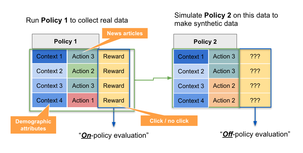
The exploration policy (policy 1) is the policy that was used to generate the historical data, while the target policy (policy 2) is the new policy for which we are trying to estimate the expected reward.
A further point of distinction to make is between stationary and nonstationary policies. A stationary policy is one which depends only on the current context, and where the probabilities for receiving different actions for a given context remain constant over time. For example, uniform random allocation is a stationary policy. In contrast, a nonstationary policy is one which depends on the current and historical contexts, where the probabilities for receiving different actions for given context change over time. Typically, this occurs because the algorithm is updating its internal model with online learning. For example, Thompson sampling is a nonstationary policy. Due to the interactive learning that is inherent to nonstationary policies, there are separate approaches to evaluating stationary and nonstationary policies.
Evaluating stationary policies
The current best practice for evaluating stationary policies is called doubly robust off-policy evaluation [2], so-called because it is based on two separate techniques that guard against each other’s weaknesses. These basis techniques are called direct method and inverse propensity score.
Direct method
The direct method involves training a model on the historical data to predict the reward for each context-action instance. In this model, the reward is the target variable, while the context and action are the input features. Using this model, we can predict the rewards for each context-action instance associated with the target policy. This is illustrated below.
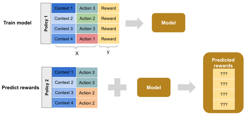
The expected average reward is the sum of the predicted rewards divided by the number of historical instances.
While this technique is straightforward, it can be highly biased, due to bias in the model and in the historical data logged by the exploration policy. For example, if a particular action was rarely selected by the exploration policy, then reward predictions for this action in the resulting model will be inaccurate. This problem is exacerbated if there is a large difference between exploration and target policies.
Inverse propensity score
One way to correct for the bias due to the difference between exploration and target policies is to re-weight each historical instance by its probability of occurring under the exploration policy.
With this technique, a synthetic dataset is created, which only contains instances where the recommended actions from the exploration policy and target policy match (by chance). Instances where they do not match are discarded. This synthetic dataset represents counterfactual results, as they approximate what would have happened if the target policy had been deployed. However, a correction needs to be applied to this dataset, due to the aforementioned difference between exploration and target policies. This correction is applied by dividing the reward of each instance by the probability of occurring under the exploration policy (or multiplying by its inverse propensity). This is illustrated below.
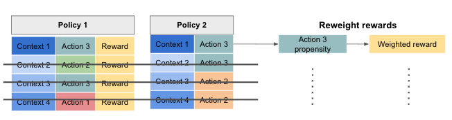
The expected average reward is sum of the re-weighted rewards divided by the number of historical instance (not just the ones with matching actions).
While this technique is unbiased, it uses the historical data inefficiently, because instances where the actions under exploration and target policies do not match must be discarded. The resulting synthetic dataset tends to be much smaller than the historical dataset, which results in higher uncertainty (variance) in the corresponding reward estimates.
Doubly robust
The doubly robust technique combines the direct method with inverse propensity scores. An intuitive way to think about it is to consider that it uses the predicted rewards from the direct method, and if there is additional information (i.e. exploration and target policy actions match) then the inverse propensity score correction is applied. This is illustrated below.
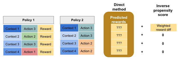
This technique is doubly robust, because if either the direct method or the inverse propensity score component is accurate, then the final reward estimate is accurate.
Evaluating nonstationary policies
The preceding sections referred to evaluating stationary policies (which depend only on current context). However, many decision-making algorithms perform online learning, where an internal model is continuously updated. Such policies are nonstationary, because they depend on the history of contexts, as well as the current context. These policies are more difficult to evaluate, because of their interactive nature.
The current best practice for evaluating nonstationary policies is called doubly robust nonstationary, as it extends the doubly robust technique described in the previous section [3]. The nonstationarity is handled by replaying the target policy iteratively over the historical data with rejection sampling, which is a way to simulate data from an unknown distribution. The technical details of this technique are beyond the scope of this blog post, but we describe some qualitative aspects below.
The technique works by iterating over the historical data and probabilistically accepting/rejecting instances to include in the synthetic dataset. By performing this rejection sampling iteratively over the historical data, the nonstationary policy under evaluation can be updated for each instance, thereby simulating online learning. In contrast, the techniques for stationary policies in the previous sections involved non-iterative, batch calculations on the entire historical dataset.
The rejection sampling is done in proportion to exploration and target action probabilities. Specifically, it tends to reject instances with actions that are more likely in exploration than target policies, so that the distribution of accepted instances more closely matches the target policy, rather than the exploration policy.
To minimise the variance in this technique, it efficiently uses all historical instances (accepted or rejected) in the doubly robust reward estimate. These reward estimates are averaged over each round, to further lower the variance. To control the bias in this technique, there are tunable parameters to control the level of bias in the estimate (at the cost of more or less efficient use of the historical data). The result is an evaluator that balances bias and variance, enabling nonstationary policies to be evaluated on historical data.
Summary
We have described off-policy evaluation as an important tool for testing decision-making algorithms without actually deploying them. It allows us to estimate how an untested target policy would have performed, using data collected by a different, exploration policy. The doubly robust approach can be applied to stationary policies (which depend only on current context), and can be extended to apply to nonstationary policies (which update continuously, depending on the current context as well as historical results). Such off-policy evaluation methods allow us to:
- rapidly iterate over candidate algorithms (which improves development speed), and
- test algorithms without deploying it to a live system (which improves development safety)
They are therefore useful to consider when building automated decision-making systems.