A/B testing is a simple way for companies to make design decisions under uncertainty. However, this simple approach is prone to having high ‘regret’ (i.e. the difference between the reward you achieve and the reward you could have achieved if you had made perfect decisions). In this post, we look at other approaches to make decisions under uncertainty more effectively.
Introduction
Many companies are familiar with A/B testing, where design decisions are validated through large scale online experimentation. Fewer companies, however, are familar with approaches to automate these experiments, or handle heterogenous treatment effects (i.e. different users respond differently to different interventions).
A set of apporaches, known as multi-armed bandits, offer a way to efficiently converge on the optimum variant without having to wait for the ‘final answer’ as in A/B testing. Furthermore, a special type of multi-armed bandit, called a contextual bandit, can find the right variant for each individual user. These algorithms can adapt and learn from the environment automatically, without human intervention.
Here, we compare A/B testing, multi-armed bandit, and contextual bandit approaches based on simulations of a synthetic population. To do this, we will use the contextual R package, which provides simple-to-use tools to simulate bandit algorithms.
First, we load these packages:
library(contextual)
library(knitr)
library(tidyverse)
library(magrittr)
We also define some functions we will use later on:
get_conv <- function(p, n){
  sample(x = c(1, 0), size = n, replace = TRUE, prob = c(p, 1 - p))
}


plot_cum_reward_comparison <- function(dt){
  dt %>%
    filter(t == horizon) %>%
    group_by(agent) %>%
    summarise(n = n(),
              cum_reward_mean = mean(cum_reward),
              cum_reward_sd = sd(cum_reward),
              cum_reward_se = cum_reward_sd / sqrt(n)) %>%
    ggplot(aes(x = agent, y = cum_reward_mean)) +
    geom_point() +
    geom_errorbar(aes(ymin = cum_reward_mean - 2*cum_reward_se,
                      ymax = cum_reward_mean + 2*cum_reward_se), width = 0.1)
}
Business problem
Suppose there are 2 variants (A and B) of a website feature we can show to users. Once we show a variant to a user, they either convert, or they don’t (i.e. there is a binary reward). Our task is to show a variant to each user, such that we maximise the cumulative reward over the entire user population. The process of showing variants to users and watching how they respond will help us determine which variant to show.
Defining the user population
horizon <- 400

# We assume that there are 2 contexts (d = 2)
# This is how they are split across the user population
# These probabilities should sum to 1
d_probs <- c(0.5, 0.5)

# Context 1's conversion probability distributions for the arms
d1_p <- c(0.6, 0.5)

# Context 2's conversion probability distributions for the arms
d2_p <- c(0.4, 0.7)
We assume that there are 400 users in our population. We also assume that there are two types of users (e.g. male and female), who respond differently to our variants. We will call these Type 1 and Type 2 users, and we assume that the population is evenly split across these two types. Type 1 users have the following conversion probabilties for variants A and B: 0.6, 0.5. Type 2 users, on the other hand, have conversion probabilties of 0.4, 0.7 for variants A and B.
Since our population is synthetic, we can know how each user would have responded if they were shown variant A, and if they were shown variant B (i.e. their counterfactual responses). This counterfactual knowledge is impossible in practice. Using the parameters above, we generate a synthetic population of users with the following:
user_idcontext- whether they are Type 1 or Type 2 usersconv_if_a- whether or not they would convert if they were shown variant Aconv_if_b- whether or not they would convert if they were shown variant B
This code generates the user population:
df <- tibble(user_id = seq(1:horizon),
             context = sample(x = seq(1:2), size = horizon, replace = TRUE,
                              prob = d_probs) %>% as.factor())

df_1 <- df %>% filter(context == 1)
df_2 <- df %>% filter(context == 2)

d1_conv_if_a <- get_conv(d1_p[[1]], nrow(df_1))
d1_conv_if_b <- get_conv(d1_p[[2]], nrow(df_1))

d2_conv_if_a <- get_conv(d2_p[[1]], nrow(df_2))
d2_conv_if_b <- get_conv(d2_p[[2]], nrow(df_2))

df_1 %<>% mutate(conv_if_a = d1_conv_if_a)
df_1 %<>% mutate(conv_if_b = d1_conv_if_b)

df_2 %<>% mutate(conv_if_a = d2_conv_if_a)
df_2 %<>% mutate(conv_if_b = d2_conv_if_b)

df <- bind_rows(df_1, df_2) %>% arrange(user_id)

df %>% glimpse()
## Observations: 400
## Variables: 4
## $ user_id   <int> 1, 2, 3, 4, 5, 6, 7, 8, 9, 10, 11, 12, 13, 14, 15, 16,…
## $ context   <fct> 1, 1, 1, 1, 2, 2, 1, 1, 1, 1, 2, 1, 1, 1, 2, 2, 2, 1, …
## $ conv_if_a <dbl> 1, 0, 1, 1, 1, 0, 0, 1, 0, 1, 1, 0, 1, 1, 0, 1, 1, 0, …
## $ conv_if_b <dbl> 1, 1, 0, 0, 1, 0, 1, 0, 0, 1, 1, 0, 1, 0, 1, 1, 1, 0, …
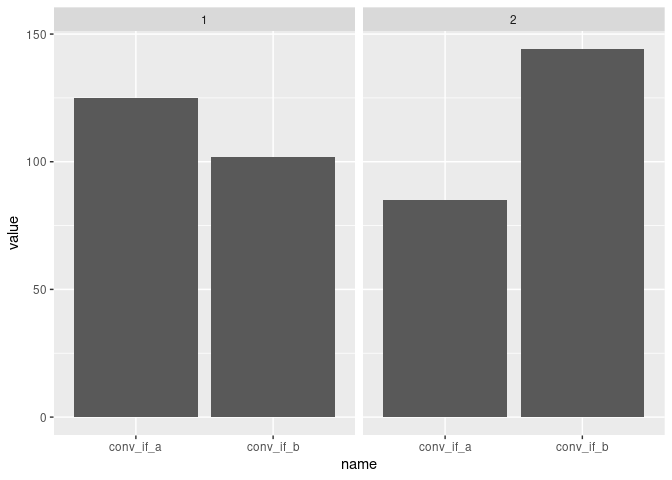
This table shows the population breakdown over context (i.e. whether the user is Type 1 or Type 2) and counterfactual responses.
df %>%
  group_by(context, conv_if_a, conv_if_b) %>%
  summarise(n = n()) %>%
  kable()
| context | conv_if_a | conv_if_b | n |
|---|---|---|---|
| 1 | 0 | 0 | 41 |
| 1 | 0 | 1 | 33 |
| 1 | 1 | 0 | 56 |
| 1 | 1 | 1 | 69 |
| 2 | 0 | 0 | 36 |
| 2 | 0 | 1 | 80 |
| 2 | 1 | 0 | 21 |
| 2 | 1 | 1 | 64 |
This plot shows the distributions of counterfactual responses for each context.
df %>%
  group_by(context) %>%
  summarise(conv_if_a = sum(conv_if_a),
            conv_if_b = sum(conv_if_b)) %>%
  pivot_longer(-context) %>%
  ggplot(aes(x = name, y = value)) +
  geom_col() +
  facet_wrap(~ context)

This synthetic user population forms our input to the bandit simulation demo. Note that this population can be swapped out and replaced with any population consisting of different contexts and counterfactuals.
Defining the bandit simulation
Get arm probabilities
The bandit simulation needs a matrix of probabilities for each arm k and context d. We can calculate these probabilties from the synthetic user population (notwithstanding the fact that we set these probabilties when we created the user population in the first place).
The matrix of probabilities looks like this:
click_probs <- df %>%
  group_by(context) %>%
  summarise(mean_conv_if_a = mean(conv_if_a),
            mean_conv_if_b = mean(conv_if_b)) %>%
  select(mean_conv_if_a, mean_conv_if_b) %>%
  as.matrix()

signif(click_probs, 3) %>% kable()
| mean_conv_if_a | mean_conv_if_b |
|---|---|
| 0.628 | 0.513 |
| 0.423 | 0.716 |
| where each row is | a context, and each column is an arm. |
Setup the bandit
This is the code to set up the bandit parameters.
# Number of bootstrap samples
simulations <- 20000

# Bandit hyperparameters
ef_epsilon <- 0.25
eg_epsilon <- 0.25
lucb_alpha <- 0.6

# Bandit
context_bandit <- ContextualBernoulliBandit$new(weights = click_probs)

# Policies
ef_policy <- EpsilonFirstPolicy$new(epsilon = eg_epsilon, N = horizon)
eg_policy <- EpsilonGreedyPolicy$new(epsilon = ef_epsilon)
lucb_policy <- LinUCBDisjointPolicy$new(alpha = lucb_alpha)

# Agents
ef_agent <- Agent$new(ef_policy, context_bandit)
eg_agent <- Agent$new(eg_policy, context_bandit)
lucb_agent <- Agent$new(lucb_policy, context_bandit)

agents <- list(ef_agent, eg_agent, lucb_agent)

# Simulator
simulator <- Simulator$new(agents, horizon, simulations, save_context = TRUE)
Our bandit simulation will run 210^{4} bootstrap simulations in parallel for each of the following approaches:
A/B testing, which is implemented with the
EpsilonFirstPolicy. This will randomly allocate variants to each user for the first 100 users, before picking the winning variant (i.e. the one with the highest conversion rate) and showing it to all the remaining users.Multi-armed bandit, which is implemented here with the
EpsilonGreedyPolicy. For each user, there is a 0.25 probability that it will show a random variant, and a 0.75 probability that it will show the currently winning variant.Contextual bandit, which is implemented here with the
LinUCBDisjointPolicy. This refers to the LinUCB algorithm. This fits a linear model for each arm, using the context as features and the reward as the label. This model is used to predict the reward and confidence bounds for each arm, given a context. The arm with the highest Upper Confidence Bound (UCB) is then chosen.
Now that we have all we need to run the simulator, we run it with this command:
history <- simulator$run()
history_df <- history$get_data_table() %>% as_tibble()
Simulation results
Cumulative reward
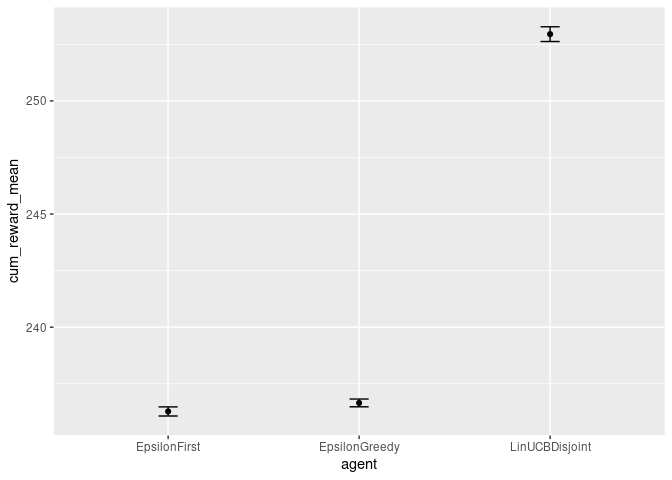
Within each approach, the bootstrap simulations all differ slightly, due to their probabilistic nature. The mean cumulative reward (and its error) is calculated for each approach over its bootstrap simulations, and plotted here:
history_df %>% plot_cum_reward_comparison()

This plot shows that the contextual bandit outperforms both the A/B testing and multi-armed bandit approaches. This is due to the fact that the user preference for variant A or B depends on the context (i.e. whether they are Type 1 or Type 2). The contextual bandit is able to use this information to make better decisions, whereas the A/B testing and multi-armed bandit approaches are blind to this.
Average reward
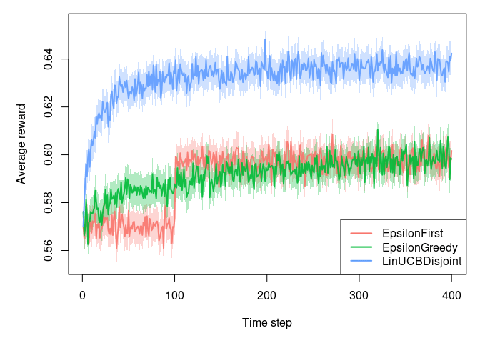
We can also plot the average reward for each approach over time:
plot(history, type = 'average', regret = FALSE, legend_position = 'bottomright', disp = 'ci')

For A/B testing (EpsilonFirst), we see a distinct step change at 100. This is where the winning variant is decided and then chosen exclusively for the remainder of the run. The multi-armed bandit (EpsilonGreedy) overtakes the A/B testing approach earlier on, which highlights the ability of the multi-armed bandit to converge to the wining variant more quickly, without having to wait for the ‘final answer’ as in A/B testing. The contextual bandit (LinUCBDisjoint) outperforms both of the other approaches, due to its ability to detect the two types of users in this population, and their differing response probabilities with respect to the variants.
Conclusion
We have shown how a contextual bandit can outperform A/B testing and multi-armed bandit approaches for this simulated user population. Note that the assumptions that we have made about the different user types this population are not particularly extreme - it’s common to see real populations with more complex heterogeneous effects. This ability of contextual bandits to handle these different user behaviours makes them well-suited to real world applications. Furthermore, both the multi-armed bandit and the contextual bandit approaches are able to achieve more conversions over fewer users, making them well-suited to situations where experiments need to be run efficiently.
Photo credit: unsplash-logoMarkus Spiske
