
As the use of AI in the modern world continues to grow, the topic of XAI becomes increasingly important. In this post, the first in a two part series, we describe what XAI and IML is, why it is important and give a quick overview of some of the popular tools before discussing some of the challenges facing modellers.
Modern artificial intelligence (AI) or machine learning (ML) methods can be used to build sophisticated models that obtain fantastic prediction performance or classification accuracy in a wide range of challenging domains. However, they typically have a complex, black-box nature, that may not help us understand the data or the task any better. Explainable AI and Interpretable ML is all about making our models more transparent and interpretable, helping us answer the important questions such as:
- What is important to the model?
- Why does the model behave the way it does?
Some authors make a distinction between models that are directly interpretable and those that require explanations. Others consider the methods for constructing directly interpretable models to be a subset of techniques sitting under the umbrella concept of XAI. Whilst authors of popluar software for generating model explanations refer to them as interpretability tools. To keep things simple in this introduction, we will follow Chris Molnar’s lead and use explainability and interpretability interchangeably, but use the terms intrinsically explainable and post-hoc explainable to describe the difference between directly interpretable models and those that require additional tools for obtaining explanations. All of these terms will be discussed in more detail below.
Improving the transparency and interpretability of our models is also important for:
- Model debugging - When/where/why is the model performing poorly?
- Model improvement - Fixing structural weaknesses in the model.
- Feature engineering - Identifying what features might be useful to create for the model.
- Controlling risk - Transparent and interpretable models make it easier to understand how the model will behave on new, unseen or rare data points.
- Ensuring compliance and fairness - By understanding how and why the model makes predictions we can make adjustments to improve fairness outcomes or meet other policy requirements.
For these reasons, improving model transparency and interpretability not only helps us build safer, explainable, more performant models, but can also help build confidence and trust in the model and its output in the eyes of technical and non-technical stakeholders. This is especially important in environments where a poorly understood model could take actions that bring financial, reputational or regulatory risks.
There is a trade off between performance and explainability
The rapid adoption of machine learning models in industry over the last decade has been driven by the ability to produce models at scale that obtain increasingly accurate classifications, predictions, recommendations or even translations from one language to another. In many cases, these models can outperform humans. Whether the task is computer vision, natural language processing or utilising a contextual bandit for customer personalisation, the improved performance of machine learning methods can often be attributed to being able to fit more complex models on larger datasets. These more complex, highly parameterised models can capture far more intricate, nuanced relationships in the data including non-linearities and interactions that a simpler model would be unable to identify. The ability to find complex but reliable patterns in large datasets can mean the difference between a successful customer interaction and the customer turning to a competitor.
Unfortunately, the superior performance of the more complex models often comes at the cost of model transparency and interpretability. The more complex a model is, the more difficult it is to understand what is important to the model and why it behaves the way it does.
Three scenarios of increasing complexity
Let us consider the three simplified modelling scenarios illustrated below.
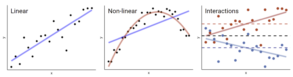
Figure 1. Three modelling scenarios of increasing complexity.
In the first scenario we may observe a clear linear relationship between the predictor and the response. Using a simple linear regression model, we can find a line of best fit, and make a general statement about how the predictor x affects the response y.
In the second scenario there is a non-linear relationship between the predictor and response. Using a simple linear model here (line in blue) would provide some predictive power, but it is clearly not a great fit. The more complicated model (line in red) fits the data very well, but our explanation for how the predictor affects the response has gotten more complicated, ‘the effect of x on y is positive, until you hit a certain value, and then the effect is reversed’.
In the third scenario there is an interaction effect between the predictor x on the x-axis and the two different groups in the data, red and blue. Here, if we did not consider the different groups, our model would conclude there is no effect of x on y (black dashed line). If we only considered the groups, we would conclude there is a difference between the two groups, but we would be unaware of the effect of the x variable. By increasing the model complexity to consider the interaction between ‘group’ and the x variable, we can find evidence that x has a negative effect on the blue group, but a positive effect on the red group.
This example illustrates that as data and modelling complexity increases, it becomes more and more difficult to explain or make general statements about the models behaviour. Even in these very simple scenarios, if we were asked the question ‘In general, what effect does increasing x have’? In anything but the simplest setting, we have to answer ‘it depends’.
Interpretability of modelling methods compared
Imagine we have a data-science task involving a very large dataset with hundreds of predictors and potentially many non-linear relationships with multi-way interactions. A simple linear model would not work well, and it would be infeasible to plot and inspect all the possible relationships in the data in an attempt to create features that capture the non-linear behaviours. The more powerful machine learning methods such as decision trees and neural networks are really good at teasing out these complex relationships but they are far less transparent and interpretable than simple linear models.
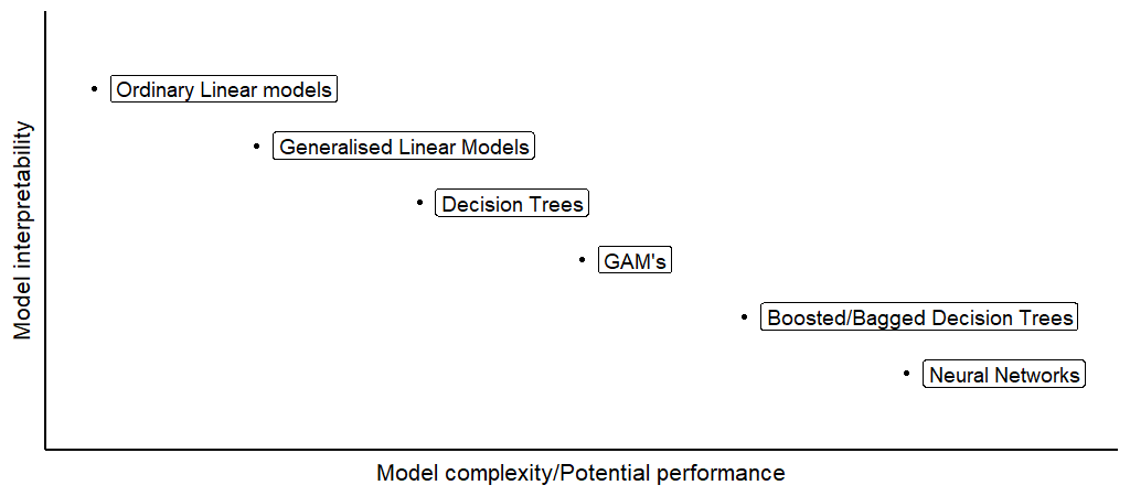
Figure 2. As the modelling methodology becomes more capable of finding complex patterns and thus more performant, the interpretability of the produced model typically drops.
Figure (2) provides a rough guide of the interpretability/complexity trade-off for a variety of very common modelling techniques. Linear models are extremely transparent and interpretable. The regression coefficients tell us directly how the predictors affect the models prediction, and simple significance tests can tell us what features are important to the model. Ordinary decision trees are more complex and can more readily handle interactions and non-linear effects. Small decisions trees can be inspected for a thorough understanding of how the decisions are made. Even with large decision trees we can still get a sense for what features are important and identify exactly the models ’reasoning’ behind any prediction.
Boosted or bagged decision tree methods such as XGBoost or Random Forest models are built from ensembles of many, often hundreds of decision trees. For these methods, it becomes infeasible to understand its reasoning directly. Without the tools discussed in the next section, it is difficult to even understand how the predictors will affect a prediction. However, we can still easily enough get a sense of what features are important to the model overall, by observing what features get used the most in the ensemble of trees, and how much information is gained by utilising them.
Neural networks are extremely popular because they are extremely flexible and can achieve state of the art performance in a wide range of modelling tasks. With enough data, increasing model complexity by adding more nodes and layers (given the right architecture, activation functions etc), we can train neural networks to identify and exploit extremely complex or nuanced relationships in data. But these networks are essentially black-boxes in terms of transparency and interpretability, making it very difficult to explain how individual predictions are made or to understand what features are important overall. Figure (3) gives a graph of a relatively simple neural net. Even in this simple network, there are a lot of stacked, non-linear transformations of the input data, making it not at all obvious how the inputs affect the outputs.
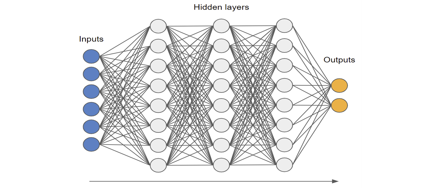
Figure 3. A diagram of a simple neural network. Provided there is enough data, complex networks are flexible enough to more easily find important non-linear relationships and interaction effects that are useful for predicting the outputs.
In some cases you might not care about how or why a prediction was made as long as it is accurate. This is common in situations where the costs of being wrong are low, such as using a recommender system to suggest movies to a user. In other cases, understanding either what is important to the model or how the model is generating its predictions might reveal useful, actionable insights about the problem. Consider a customer churn prediction model, understanding why the model predicts a customer might churn might provide insight into how to prevent customers from churning in the first place.
Fortunately, methods for explaining and understanding complex AI/ML models have received significant attention over the last few years. Powerful techniques and tools have been developed to give model builders the ability to shine some light and understand what is going on inside even the most complex black-box models.
How to think about explaining machine learning models
Before looking at specific techniques for explaining ML models, it will be helpful to build a vocabulary that will help us think about what we can explain and how we may go about it. This helps us consider what type of explanations we want and what methods are compatible with the model we have trained:
- Intrinsically explainable - An intrinsically explainable model is designed to be simple and transparent enough that we can get a sense for how it works by looking at its structure, e.g. simple regression models and small decision trees. These models are directly interpretable.
- Post-hoc explainable - For more complicated, already trained models, we can use explainability tools (often called interpretability tools) to obtain post-hoc explanations. Explanations of sufficiently complex models such as deep neural networks are always post-hoc explanations as they are not directly interpretable.
The types of ‘explanations’ typically fall into one of two categories:
- Global explanations - A global explanation of a ML model details what features are important to the model overall. This can be measured by looking at effect sizes or determining which features have the biggest impact on model accuracy. Global explanations are helpful for guiding policy or finding evidence for, or rejecting a hypothesis that a particular feature is important. Figure (4) shows a visualisation of a global explanation for a wine classification task.
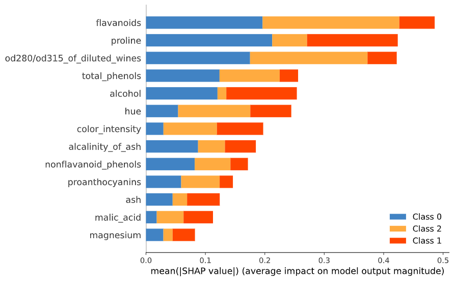
Figure 4. An example of a global explanation for a multi-class classification problem. The size of the horizontal bars indicate how much each feature (on average) influences the classification of a wine into one of three classes.
- Local explanations - A local explanation details how a ML model arrived at a specific prediction. For tabular data, it could be a list of features with their impact on the prediction. For a computer vision task, it might be a subset of pixels that had the biggest impact on the classification. Figure (5) shows an example of some local explanations for model predictions for three unique instances. Local explanations are useful for deep-dive insights or diagnosing issues and can provide answers to questions like:
- Why did the model return this output for this input?
- What if this feature had a different value?
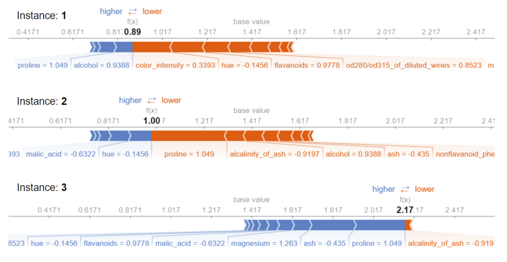
Figure 5. Local explanations of the predictions for three different instances in a wine classification task. The local explanations give the direction and magnitude each feature has on the model output relative to the baseline.
Some methods are a mix of both, providing detailed explanations of how a single feature or interaction of two features impacts a set of predictions. These are modular global explanations because they can only be used to inspect the impact of one or two features at a time.
The methods used to provide explanations are either model-specific or model-agnostic:
- Model-specific - Model-specific methods work by inspecting or having access to the model internals. Interpreting regression coefficient weights or P-values in a linear model or counting the number of times a feature is used in an ensemble tree model are examples of model-specific methods.
- Model-agnostic - Model-agnostic methods work by investigating the relationship between input-output pairs of trained models. They do not depend on the internal structure of the model. These methods are very useful for when we have no theory or other mechanism to interpret what is happening inside the model.
Some interpretability tools are described as example-based. These are model-agnostic and use the difference or similarity between examples in the data to provide an understanding of how the model behaves. Example-based explanations can provide intuitive explanations for predictions when the features in the data are simple or human-interpretable.
The choice in the interpretability tools we can apply will depend on the class of model we have trained, and the type of data we are using. Some tools are only suitable for classification tasks, some cannot handle categorical inputs, others have little restrictions but can be very computationally expensive.
The tools for explaining machine learning models
Below we list some of the popular techniques for explaining ML models, varying in complexity, applicability and the type of information they provide.
| Technique | Local | Modular Global | Global | Model-specific | Model-agnostic | Example based |
|---|---|---|---|---|---|---|
| Partial Dependence Plots [PDP] | ✓ | ✓ | ||||
| Individual Conditional Expectation [ICE] | ✓ | ✓ | ||||
| Accumulated Local Effects [ALE] | ✓ | ✓ | ||||
| Anchors [ANC] | ✓ | ✓ | ||||
| Permutation Feature Importance [PMP1, PMP2] | ✓ | ✓ | ||||
| Integrated Gradients [IG] | ✓ | ✓ | ||||
| Local interpretable model-agnostic explanations [LIME] | ✓ | ✓ | ||||
| Kernel SHAP [SHAP] | ✓ | ✓ | ✓ | |||
| Tree SHAP [TSHAP] | ✓ | ✓ | ✓ | |||
| Counterfactual Explanations [CE] | ✓ | ✓ | ✓ | |||
| Prototype Counterfactuals [PC] | ✓ | ✓ | ✓ | |||
| Adversarial Examples [AE] | ✓ | ✓ | ✓ |
We find PDP and ICE plots to be useful for investigating the impact that specific features have on model predictions and Kernel SHAP to be extremely useful for generating easy to interpret local and global explanations for black box models. Figure (6) shows a PDP with ICE curves and figures (4) and (5) show examples of how global and local explanations can be rendered from a Kernel SHAP explanation.
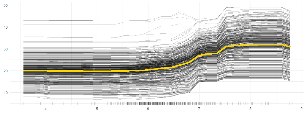
Figure 6. A PDP + ICE plot. The yellow line (PDP) shows the marginal effect of the predictor on the model output as the feature on the x axis is varied, everything else being equal. The individual black lines (ICE) show the effect of the predictor on all of the individual instances in the data. The yellow line shows us that whilst increasing x typically has a positive impact on y, the black lines show us that (possibly due to interactions with other variables) increasing x can have a negative effect on some instances.
Adversarial examples are a particularly interesting tool, not for understanding how the model works but for understanding how they can be forced to fail. For more information on many of these methods please see the references below or take a look at Chris Molnar’s excellent book, Interpretable Machine Learning [IML].
Some discussion points
What we can and cannot explain with XAI tools
So far we have discussed how and why explainable machine learning is beneficial and the types of questions that can be answered using the popular interpretability tools. But we must also take a moment to think about the kind of questions these tools cannot answer, but might be expected to by non-practitioners.
We have to remember that the algorithms we typically use to train machine learning models are not optimised for being interpretable, understandable or even building an accurate representation of reality, they merely optimise a loss function. We can only attempt to explain why the model generates the predictions it does, not the reasons for why one value of a feature has a larger effect than another unless we have a physical, causal model of reality. Because XAI tools can provide us with effect sizes, it can be very tempting to give them a causal interpretation.
Consider a model that predicts the top speed of a car based only on it’s colour, the number of doors it has and if the car is a convertible/cabriolet. Using XAI tools we can understand how important each variable is and the effect of each variable in the generation of each prediction to the point where we can get a good understanding of how the three variables interact. However, these tools aren’t telling us why some cars are faster than others, they are simply ‘explaining’ how the predictions were generated. We might find that the model estimates the highest top speed belongs to green convertibles with two doors. The reason why the model estimates that green two door convertibles have the highest top speed is because cars fitting that description in the dataset were mostly modern Lamborghini’s that have very powerful engines and predicting a high top speed for this cohort minimised the loss function we selected. Figure (7) provides the data generation process for this scenario, with the observed variables in the blue box. There is no causal relationship between colour and top speed, only an observed correlation. If however, we did observe ‘engine power’, we could rightly attribute a causal effect between it and top speed.
Caution must be taken to avoid causal interpretation when it is not valid. (Green cars are not inherently faster than red ones so it is not the case that painting a car green will make it faster.)
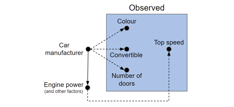
Figure 7. The car manufacturer determines the colour, number of doors, whether the car is a convertible or not and the top speed. But in our dataset we only observe the variables in the blue box where there are no arrows between the predictors and top speed.
Other limitations
Explainability of complex black-box models is not a flawless procedure. The tools used to explain black-box models typically involve the construction of an understudy model that is likely not perfect and can sometimes produce very misleading explanations, potentially not even matching the prediction produced by the original model. Cynthia Rudin recommends building intrinsically explainable or directly interpretable models for high-stakes decision making.
It also might be the case that some sufficiently complex models whilst incredibly useful and predictive, just escape a truly human-interpretable explanation. Keith O’Rourke paraphrases Stephen Wolfram on this topic.
If we choose to interact only with systems that are computationally much simpler than our brains, then, yes, we can expect to use our brains to systematically understand what the systems are doing … But if we actually want to make full use of the computational capabilities that our universe makes possible, … we’ll never be able to systematically ‘outthink’ or ‘understand’ those systems … But at some level of abstraction we know enough to be able to see how to get purposes we care about achieved with them.
Is it the data and not the model that needs to be explained?
Sometimes, we are asked to explain why the predictions being generated from a model are different in distribution from those observed in the past. Perhaps our model is recommending scarves and winter gloves instead of t-shirts and swimsuits. By inspecting our global model explanation we might observe that ‘season’ is an important feature and conclude that transitioning from Summer to Autumn has a significant impact on people’s behaviour. Here, it might be obvious that the input data that has changed and explains the change in model output.
Now, say the conversion rate has dropped for our product recommendation model. On the surface this may feel like another ‘explain the model’ problem, but consider the case where a stage in our ML pipeline breaks, perhaps the data stops being recorded properly and the ‘age’ feature gets set to a default value of NA or 0. Very likely, our model will start recommending products to adults that they do not want and conversion rates will suffer. With some work we could use the XAI tools and inspect a bunch of predictions to understand why the performance is dropping. But it would be far easier to resolve this issue by employing tools to detect changes in the distributions of the input data than it is to investigate the model outputs. Here, the XAI tools can only help us indirectly.
Are open and totally transparent models always good?
Transparent models can reveal their inner workings and provide us with a better understanding of the world, but there are some use-cases where models should only be made transparent to a limited number of people. Totally open and transparent models are open to exploitation and being gamed. Consider the following examples:
- Search engine listings - If a search engine’s algorithm was open to everyone, the recommended websites at the top of each query would likely just be those that best exploited the model, not the website people generally want to visit.
- Credit applications - If the decision rules for credit and loan applications were exposed, banks and creditors would end up loaning money to individuals who would be unlikely to repay them in full.
- Self-driving cars - Using adversarial examples, a nefarious actor could trick the AI behind a self-driving car to have an accident.
Summary and a preview of part two
Thanks for reading this introduction to Explainable AI. In this post we:
- Considered how improving model interpretability can allow us to build better, safer, more trusted models.
- Demonstrated that interpreting and explaining models and their predictions gets more difficult as models get more complex.
- Explained the important concepts that are essential for understanding Explainable AI and interpretable ML methods and tools.
- Explored a variety of popular tools and illustrated how they can help us understand our models.
- Discussed some of the limitations of Explainable AI.
In our next blog post on this topic, we will take a look at how we use XAI tools at Ambiata to open up and explain complex contextual bandits for continuously learning models. We will discuss:
- A quick overview of contextual bandits.
- What is different about XAI in the context of continuously learning models.
- Explaining historical behaviour and future behaviour.
- Explaining bandit predictions and bandit actions.
Learn more
Do you need some help in evaluating your algorithms, determining what is important to the model and explaining why the model behaves the way that it does? If so, Ambiata provides consulting services on these topics. Please feel free to contact us at info@ambiata.com or on the web form on our main page.
References
- [PDP] Friedman, Jerome H. “Greedy function approximation: A gradient boosting machine.” Annals of statistics 2001.
- [ICE] Goldstein, Alex, et al. “Peeking inside the black box: Visualizing statistical learning with plots of individual conditional expectation.” Journal of Computational and Graphical Statistics 24.1 2015.
- [ALE] Apley, Daniel W. “Visualizing the effects of predictor variables in black box supervised learning models.” arXiv preprint arXiv:1612.08468 2016.
- [ANC] Marco Tulio Ribeiro, Sameer Singh, Carlos Guestrin. “Anchors: High-Precision Model-Agnostic Explanations.” AAAI Conference on Artificial Intelligence (AAAI), 2018.
- [PMP1] Breiman, Leo. “Random Forests.” Machine Learning 45 (1). Springer. 2001.
- [PMP2] Fisher, Aaron, Cynthia Rudin, and Francesca Dominici. “Model Class Reliance: Variable importance measures for any machine learning model class, from the ‘Rashomon’ perspective.” http://arxiv.org/abs/1801.01489 (2018).
- [IG] Sundararajan, Mukund, Ankur Taly, and Qiqi Yan. “Axiomatic attribution for deep networks.” International Conference on Machine Learning. PMLR, 2017.
- [LIME] Ribeiro, Marco Tulio, Sameer Singh, and Carlos Guestrin. “Why should I trust you?: Explaining the predictions of any classifier.” Proceedings of the 22nd ACM SIGKDD international conference on knowledge discovery and data mining. ACM (2016).
- [SHAP] Lundberg, Scott M., and Su-In Lee. “A unified approach to interpreting model predictions.” Advances in Neural Information Processing Systems. 2017.
- [TSHAP] Lundberg, Scott M., Gabriel G. Erion, and Su-In Lee. “Consistent individualized feature attribution for tree ensembles.” arXiv preprint arXiv:1802.03888 (2018).
- [CE] Wachter, Sandra, Brent Mittelstadt, and Chris Russell. “Counterfactual explanations without opening the black box: Automated decisions and the GDPR.” (2017).
- [PC] Van Looveren, Arnaud, and Janis Klaise. “Interpretable Counterfactual Explanations Guided by Prototypes.” arXiv preprint arXiv:1907.02584 (2019).
- [AE] Szegedy, Christian, et al. “Intriguing properties of neural networks.” arXiv preprint arXiv:1312.6199 (2013).
- [IML] Molnar, Christoph. “Interpretable machine learning. A Guide for Making Black Box Models Explainable”, 2019. https://christophm.github.io/interpretable-ml-book/.
- [RUDIN] Rudin, C. Stop explaining black box machine learning models for high stakes decisions and use interpretable models instead. Nat Mach Intell 1, 206–215 (2019).