
We show how the deployment design pattern for continuous intelligence systems differs from those used in traditional ML.
In the previous post 1, we built out the data access components of the architecture and outlined our two layer API approach that enables both data enrichment, and traffic routing to different recommendation methods.
Now, in part three of our series on next-best-action systems, we will compare deployment design patterns for machine learning methods, and show how continuous intelligence systems differ from those used in traditional ML. All decision-making algorithms learn from input data, but there are different ways in which algorithms can process it, and the best approach depends on the problem type. Specifically, we will look at how the deployment design pattern for continuous intelligence differs from traditional ML.
In this discussion, we assume that data is comprised of data instances, which are the individual examples (e.g. rows) of data used for model training and prediction. Actions are the available interventions that the next-best-action system has to choose from, to recommend for each data instance. Traditional ML refers to the typical ML projects where supervised learning models are trained using batches of data (i.e. some number of instances). In contrast, continuous intelligence refers to ML projects that operate on a continuous feedback loop, like reinforcement learning or multi-armed bandit algorithms.
Traditional ML deployment
The figure below shows a deployment design pattern for traditional ML.
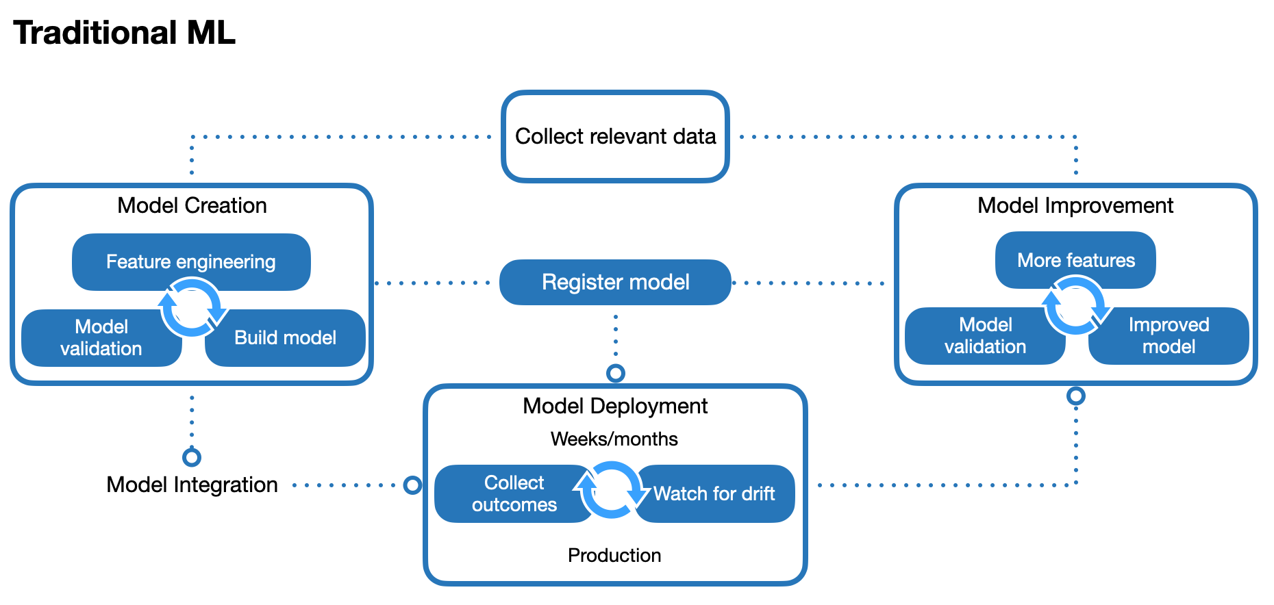
In this design pattern, an initial batch of historical data is collected and used for the model creation process, which is comprised of feature engineering, model building, and model validation. By training the model on historical data with known outcomes, it can be used to make predictions on new data with unknown outcomes. Once the model is deployed in production, the actual outcomes are monitored over time to check for dataset shift 2, which occurs when the training data or model is no longer representative of the current environment, causing model performance to degrade over time. In typical business applications, it can take weeks or months to detect dataset shift.
This design pattern has a model improvement process to periodically retrain the model if dataset shift occurs (or as better data or models become available). Model improvement may require collecting more data for additional features, or other changes to the model, before the model is redeployed. A centralised model registry tracks model versions throughout the various development and production phases, for all models used across the organisation. The traditional ML deployment design pattern has become the de-facto standard in many business ML applications.
Note that the traditional ML design pattern assumes that models are created and improved using batch learning (also called offline learning), where ML models are trained on batches of data. In this design pattern, the model can only be created or improved once a batch of data has been collected.
For next-best-action systems, each action’s probability of being recommended (given some data input) is called the policy. With the traditional ML design pattern, this policy remains fixed until the model itself is updated, and is referred to as a stationary policy.
Continuous intelligence deployment
In contrast, the figure below shows a deployment design pattern for continuous intelligence (differences from the traditional ML deployment emphasised).
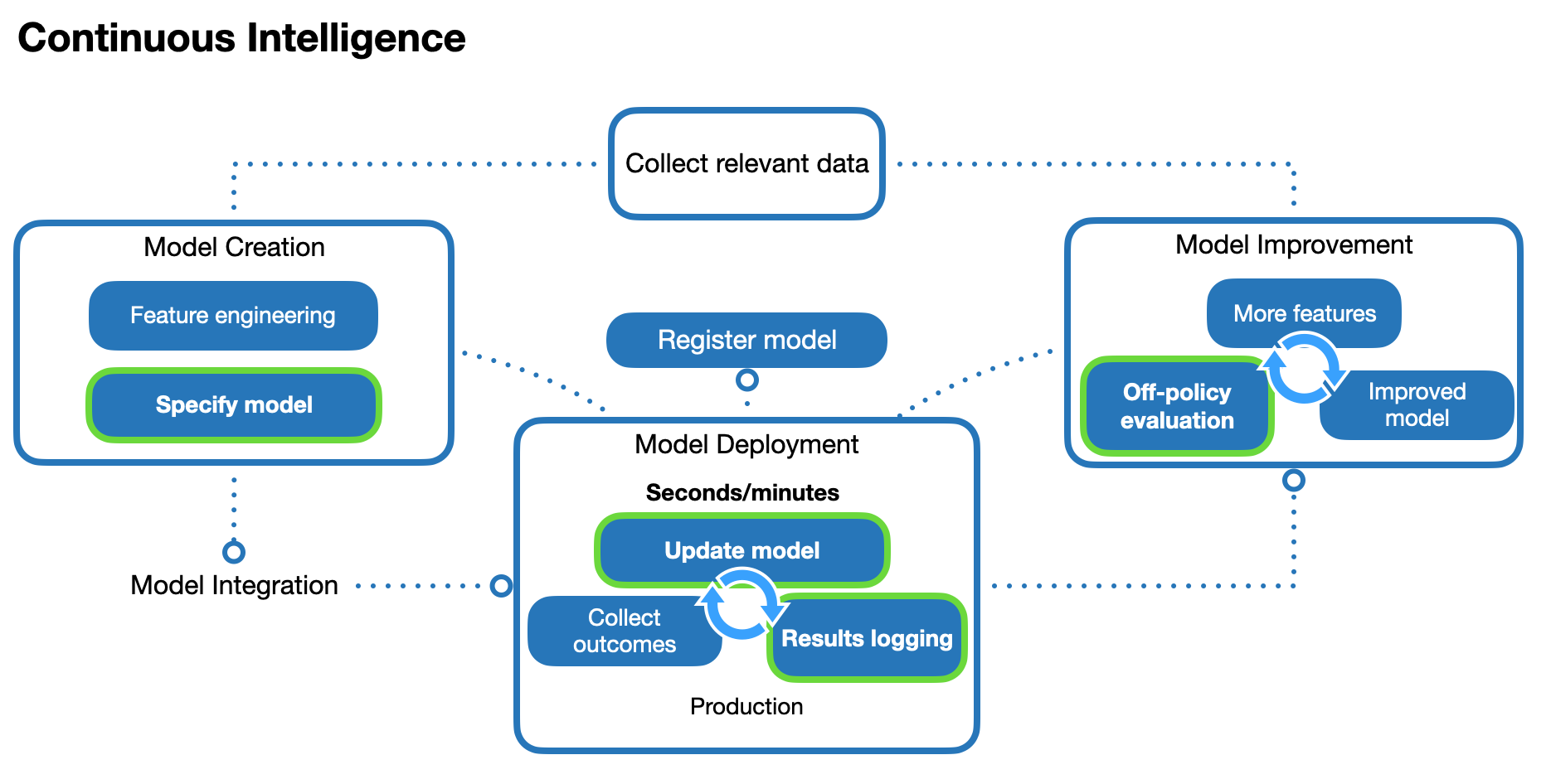
As with the traditional ML deployment, there are model creation, improvement, and deployment processes, along with a centralised model registry for model version tracking. However, instead of the batch learning, this design pattern uses incremental learning (also called online learning), where models are incrementally updated as the data is collected. These model updates occur continuously as each new data instance arrives. We can think of incremental learning as a special case of batch learning where retraining occurs after each additional data instance. This learning cycle typically takes seconds or minutes in typical business applications. In the context of next-best-actions, we refer to this as a non-stationary policy, because the policy (each action’s probability of being recommended, given some data input) changes over time as the model continuously updates.
There is a distinction here between the model improvement and model update processes. A model improvement is a general change to the model structure, for example, by adding or removing features. A model update is a special case of a model improvement that keeps the model structure unchanged, and only updates the values of the internal parameters using new data instances. For both traditional ML and continuous intelligence design patterns, model improvement occurs as a separate process. However, the model update process differs between the two design patterns. In a traditional ML deployment, model updates can only occur after a new batch of data instances has been collected, as part of a model improvement process. In a continuous intelligence deployment, the model is updated continuously in production after it has been deployed.
For continuous intelligence deployments, the model creation process does not need a model trained on an initial batch of data (only an ongoing stream of current data). However, it needs a model to be specified in such a way that it can learn from a data input stream. This allows the deployed model to update itself in production, as it learns ‘on-the-fly’, and outcomes are collected to continuously update the model. In the context of next-best-actions, the outcomes must be logged, along with the data input, the recommended action, and the probability for recommending that action (we explain why in the next section).
Offline evaluation
For safety reasons, the performance of a next-best-action system must be evaluated prior to deployment (offline). This can be achieved through off-policy evaluation 3, which uses historically logged data to recreate counterfactual results (i.e. how a policy would have performed if it had been deployed over the period of the historical data). Off-policy evaluation techniques typically require accurate logging of the outcome, the recommended action, and the probability for recommending that action for every instance.
In traditional ML deployments, the policies are stationary (until the model is next retrained), so off-policy evaluation techniques for stationary policies 4 can be used.
However, off-policy evaluation techniques for non-stationary policies are required in continuous intelligence deployments, because the models continue to learn after deployment. It these deployments, it is common to have action probabilities that are continuously updated, so logging these probabilities for each data instance is important.
Performance over time
The figure below illustrates a hypothetical example of how deployments under the two design patterns might perform over time.
The vertical axis measures the reward, indicating how well the model is performing. The horizontal axis measures time over which input data is received. Traditional ML uses batch learning, so there is an initial period where there is no reward contribution from the model, as the input data is only being collected for the initial model training batch. When the initial model is then deployed (Batch v1), there is a jump in the reward, as it switches over from model training to making predictions with the model. However, the model performance degrades over time, as new data drifts and no longer matches the initial training batch. Once the performance worsens below a pre-specified threshold, the model is retrained on the latest data to bring the performance back up (Batch v2). Alternatively, retraining could simply occur on a regular, fixed schedule. As the cycle of performance degradation and model retraining repeats (Batch v3), the performance over time takes on a sawtooth-like pattern.
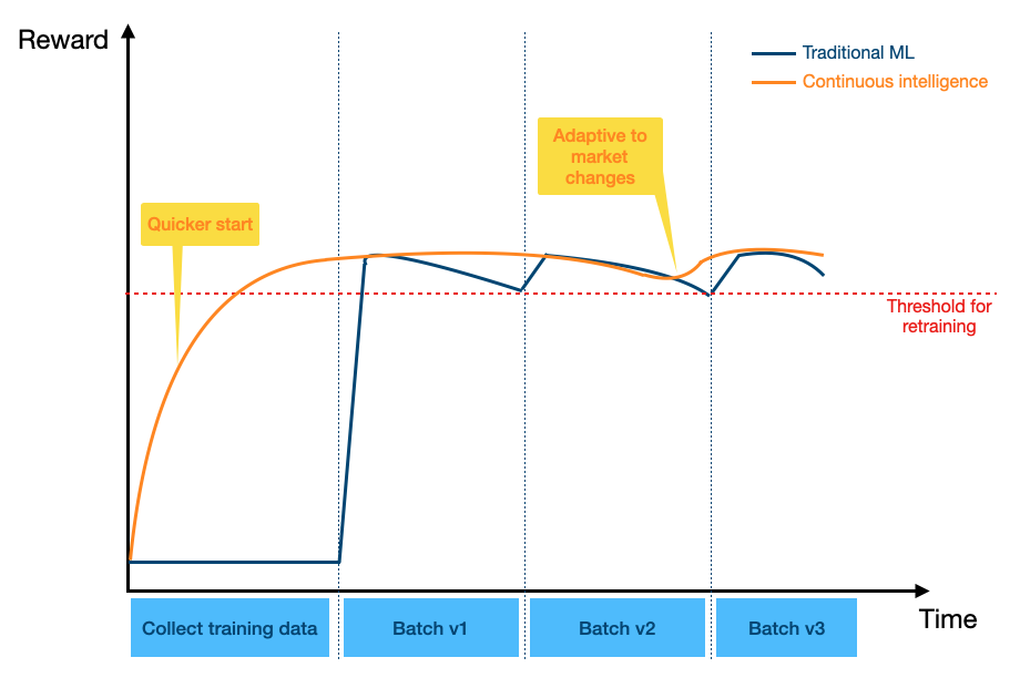
Continuous intelligence uses incremental learning, so the deployed model starts learning and improves from the start. The reward contribution from the model increases without needing to wait for an initial training batch to be collected. While the typical reward per instance is similar to that of traditional ML, it is less susceptible to dataset shift, as it is continuously updated. If there are sudden changes in the environment (e.g. change in market conditions), the continuous intelligence model adapts quickly, without requiring a full retrain of the model (only the parameter values are updated).
The areas under each curve represent the cumulative rewards for each model, and in this example, the continuous intelligence model has a higher cumulative reward than traditional ML.
Exploring next-best-actions
The continuous intelligence approach is designed to balance the explore/exploit trade-off in bandit algorithms and reinforcement learning5. Because the model updates can occur between individual instances, it has more flexibility to iteratively explore the rewards for each action (given a data input). An example of this is illustrated in the figure below. Typically, traditional ML models focus on point estimate reward predictions for each action. In the traditional ML example below, Action 1 has the highest predicted reward for a given data instance, and would therefore be the recommended action for this instance. The only way the prediction could change for this instance would be if the model were retrained. This approach of simply selecting the action of the highest predicted reward based on some initial batch training data is analogous to traditional A/B testing.
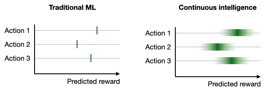
In contrast, continuous intelligence models can make better use of the uncertainty estimates around the predicted reward for each action. By calculating the probability distribution of the reward, we can recommend an action based on the probability of it being the best action. In this example, Action 1 has the highest probability for being recommended, but there is still a good chance that Action 2 or 3 could be recommended. The outcome resulting from the action recommendation would then be used to update the corresponding action’s distribution. This approach is called Thompson sampling, and has been demonstrated to be a useful approach to balancing the explore/exploit trade-off 6. While batch learning approaches in traditional ML deployments are also compatible with stochastic policies, the iterative learning cycle of continuous intelligence deployments gives them more opportunities to learn from the data and adjust accordingly.
Other considerations
Generally, continuous intelligence is more appropriate in applications where the input data instances are expected to arrive as a stream over time (e.g. visits on a website) rather than in batches. Since it can adapt to change more easily, continuous intelligence is also more appropriate if the population that the model is making predictions on is expected to change behaviour over time (as long as the behaviour change is not too sudden).
Conversely, traditional ML is more appropriate if a large, historical dataset already exists, and we expect that there will be little dataset shift over time. While dataset shift can be overcome by retraining the model, the time required for this is typically longer than the time it takes for a model update in continuous intelligence.
Although our discussion has been around two separate design patterns, it is important to note that they are not mutually exclusive. For example, it is feasible to initialise a deployment with a model trained on batch data, and continuously update the parameter values as new data arrives. Also, there is no clear boundary between batch learning and incremental learning, they exist on opposite ends of a spectrum, depending on the number data instances used to retrain and update the model.
It is also important to consider what an appropriate training dataset size is for both traditional ML and continuous intelligence deployments. This corresponds to the size of the time window used to collect data for updating the model. If this time window is too large, then there is the risk of the resulting models giving too much weight to data instances that occurred in the distant past. If the time window is too small, then there may not be enough data for the resulting models to give good performance.
Summary
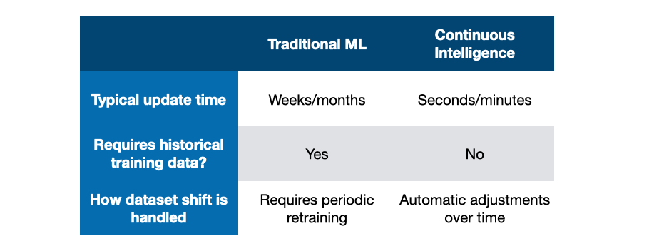
We have compared two approaches to running a next best action architecture, and described situations where one approach might be preferred over the other. Some considerations are summarised in the table below.
At Ambiata, we specialise in building and deploying applications that follow the continuous intelligence design pattern. If this sounds like something you want to do, then we’d love to hear from you.